Understanding mesh and point cloud filters

· Point Cloud Filters

There are 3 different ways to select dense point clouds filters:

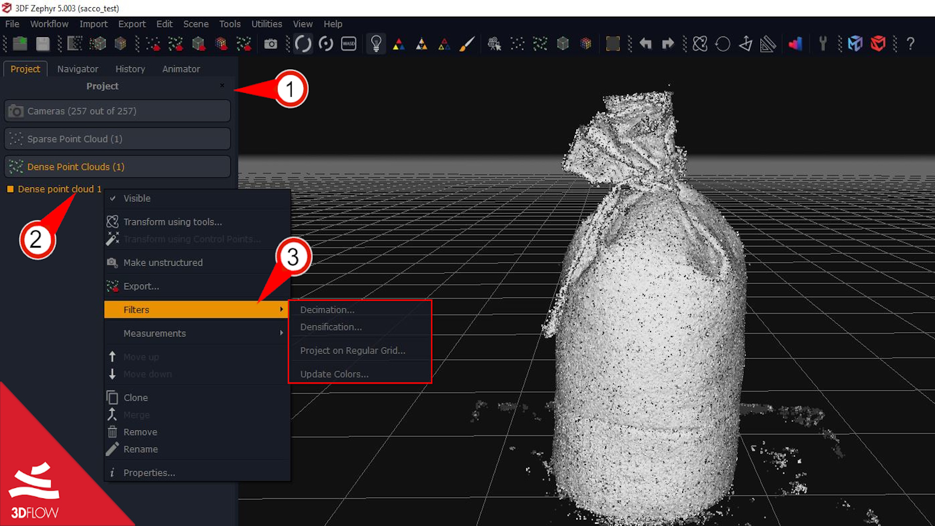
1. From the Project menu on the left (1), right-click on the created Dense point cloud name (2) and select the Filters menu (3).



 

2. From the Tools menu (1), selecting Point Cloud Filters (2).In this way, it is possible to apply filters (3) to dense point clouds in the workspace.



 

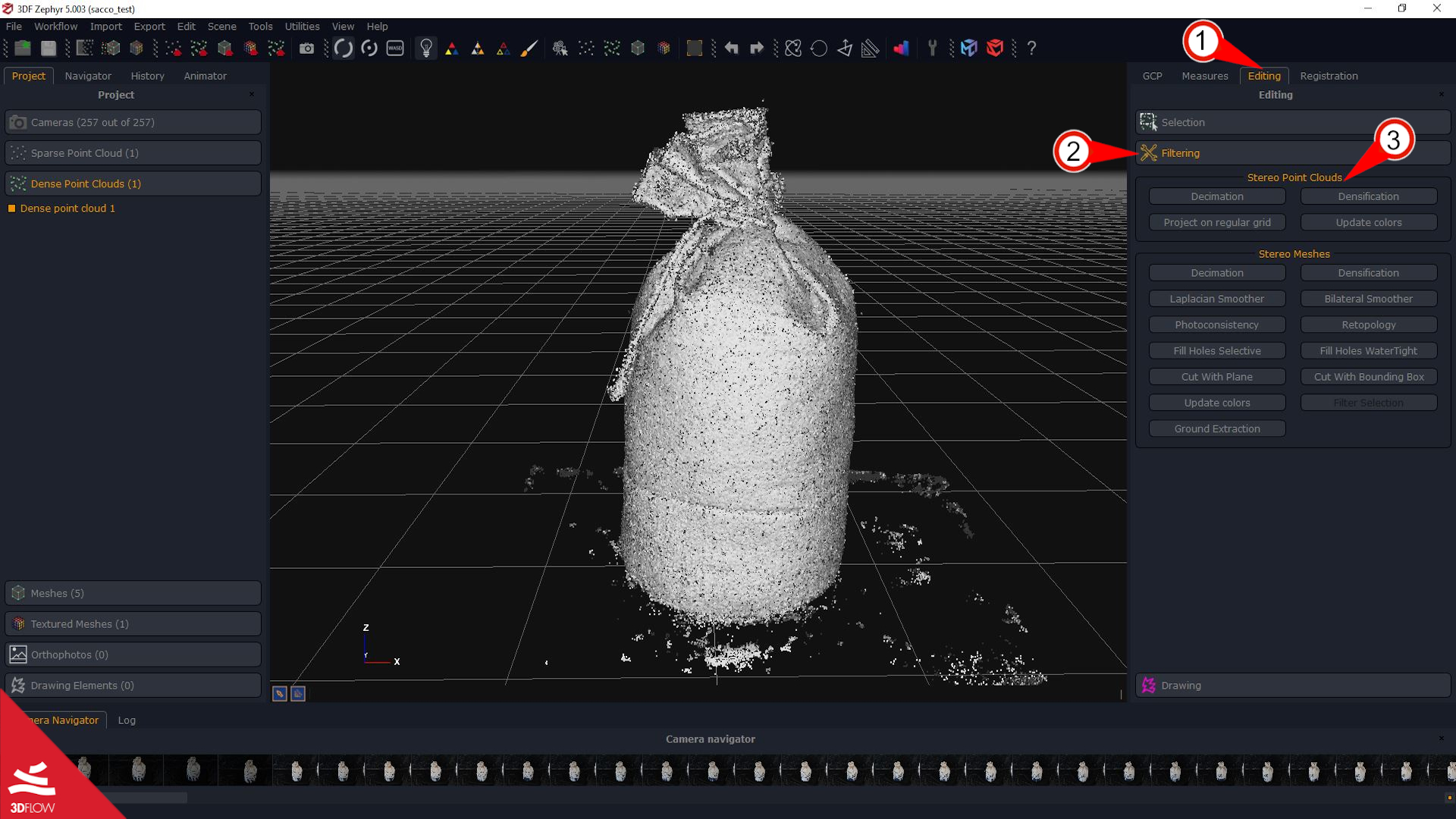
3. From the right-side context menu Editing (1), selecting Filtering (2). In the section Stereo Point Clouds (3), relative filters can be found.

Hereafter you can find a description of the different filters:

Decimation: allows selecting the desired point cloud with the dropdown menu and the number of wanted points. The point cloud will be regenerated, decimating the point count to the maximum specified value.
It is possible to decimate the desired point cloud using these different methods:

– Maximum points count;

– Maximum points count with octree (the octree is a data structure which guarantees a more homogeneous distribution of the decimated points);

– Average point distance;

– Octree size.

Once you have input the corresponding threshold for one of the Decimation filter options (target points, octree size, etc.), you can either apply the filter to the point cloud you have selected or clone that cloud and apply the filter to it. The latter one is suitable to keep the original dense point cloud and apply the filter to its copy.
 

Densification: select the desired point cloud with the dropdown menu and the number of wanted points. The point cloud will be regenerated, densifying the point count to the maximum specified value. Once you press “Apply filters”. Only structured point clouds can be densified.

Project on the regular grid: this filter leverages a regular grid as a projection for the dense point cloud so that points are at a regular distance. You can define the grid spacing as well as the grid research value for the grid generation. This tool affects surveying, mapping, mining, and construction scenarios.

Update colors: this filter allows re-computing dense point cloud colors:

– From images: (e.g., to change the workspace pictures if you are dealing with multispectral imagery).

– By elevation: it updates the colors according to the points’ elevation. A list of color maps will allow you to pick among several color palettes.

– By normals: using normal maps from the dataset images.

– Uniform: choosing one specific color from a color palette.

– By confidence: different sets of colors can be applied, depending on the confidence derived from the points targeted by the cameras..

· Mesh Filters

It’s possible to access the Mesh filters in 3 different ways:

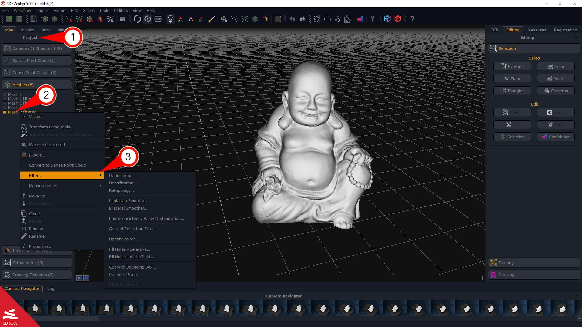
1. From the Project tab on the left (1), right-clicking on the mesh name (2) and selecting the Filters option (3).


 

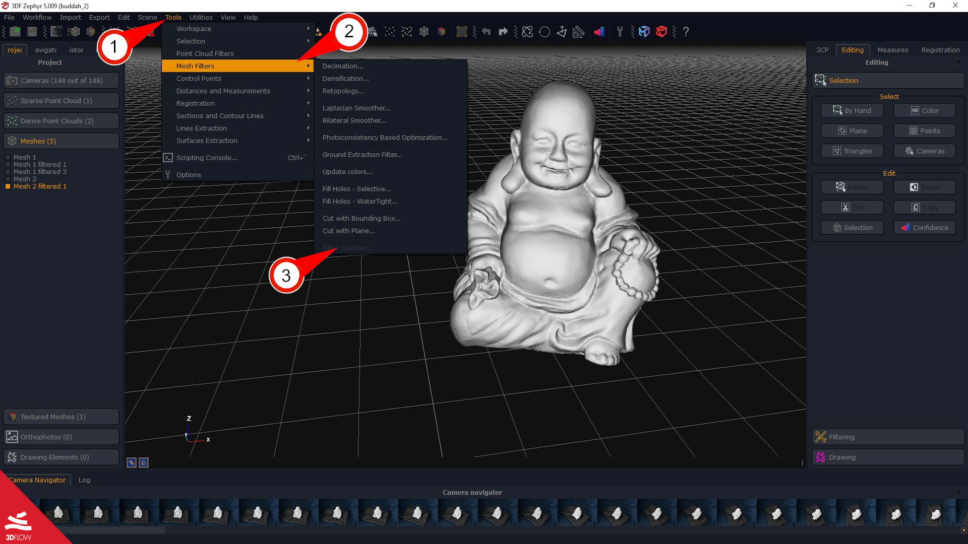
2. By clicking on Tools (1) on the bar’s menu, and selecting Mesh Filters (2). In this way, it is possible to apply the different filters (3) to meshes in the workspace.


 

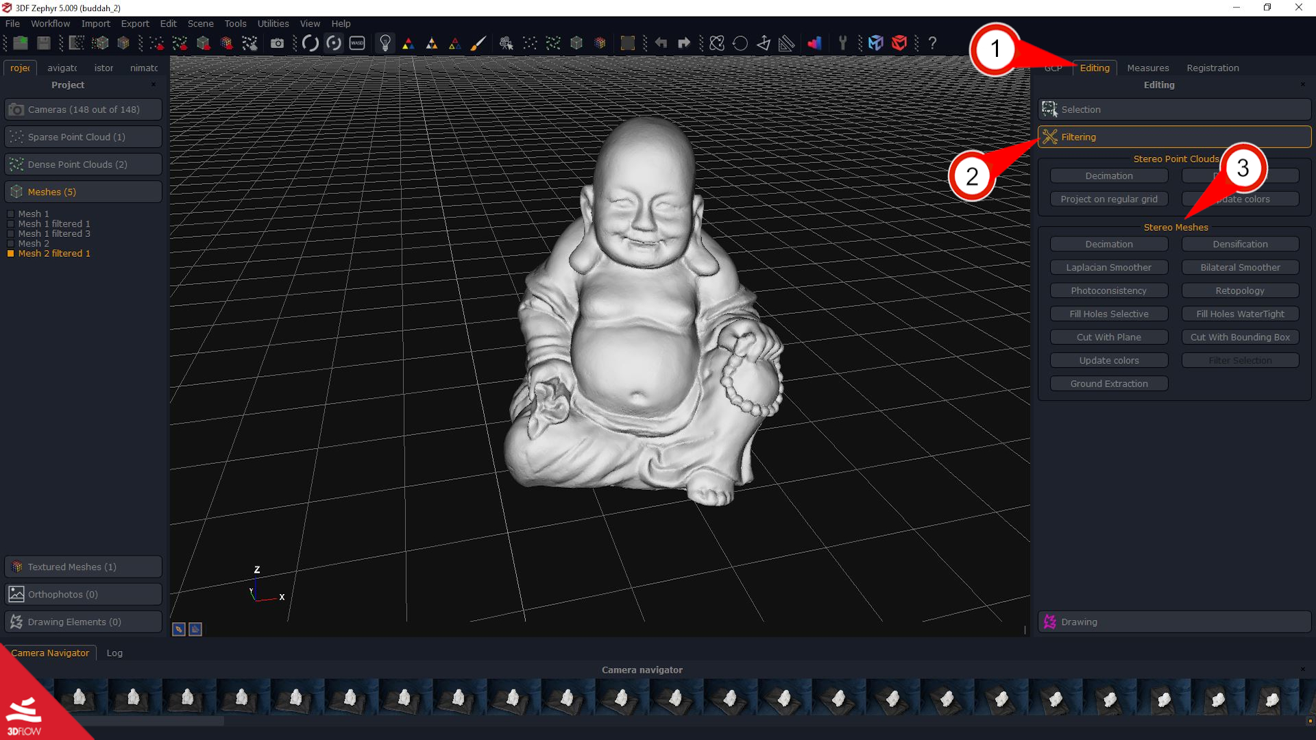
3. By selecting the Editing menu (1) and after Filtering tab (2), inside the Stereo Meshes panel (3).

The following Filters can be applied to meshes:

Decimation: allows selecting the referred mesh from the dropdown menu and setting the number of corresponding vertices. The mesh will be regenerated by decimating the number of vertices with the specified maximum value.
You can ask the software to:
– Preserve the boundaries: with this option, the vertice’s borders are never decimated. Therefore, it will allow having an edge equal to the starting mesh; the disadvantage is that the border remains much denser at the expense of the inner part, resulting in fewer points and less detail.
– Constraint distances from the input mesh: the decimation process uses an extra constraint for selecting the vertices to be decimated, which is based on the distance from the starting mesh.

You can either apply the filter to the mesh you have selected or clone it and filter the copied mesh.

Densification: select the reference mesh with the drop-down menu and the desired number of vertices. The mesh will be regenerated by densifying the number of vertices with the specified maximum value.
You can either apply the filter to the mesh you have selected or clone it and filter the mesh copy.

Laplacian smoother: reduces the mesh noise and does not keep sharp edges. The more iterations are inserted, the more smooth the mesh will be. This filter is suitable for non-edged subjects (e.g., human body datasets).

Bilateral smoother: the filter allows to smooth the selected mesh with the appropriate drop-down menu. It reduces noise by improving and emphasizing edges where it is possible. This filter is suitable for architecture and construction scenarios.

Retopology: This filter allows you to optimize the mesh topology. Triangles will be simplified and Zephyr will try to generate larger triangles where possible. The greater the optimization factor, the larger the size of the generated triangles. Please, note the Retopology filter may cause a loss of mesh detail, especially where there are geometries with well-defined edges.

Fill Holes Selective or WaterTight:
Two modes are available:
– WaterTight: allows automatically filling all the holes at once.
– Selective: allows filling the holes manually in the selection window. Users can select a specific hole by choosing the corresponding number with the pick hole button (the hole will be highlighted with an outline in the workspace) or by defining the size threshold using the dedicated slider.
The color of the triangles that will close the hole will most likely be wrong when the missing visibility of the point from the camera will behave in a degenerated way (and it is impossible to identify the color of something that is not seen by any picture). The Selective mode allows you to close single holes faster, but it may not work for complex cases, which we recommend using the WaterTight mode.

Cut with plane: this function allows you to cut the mesh sharply with a plane, regenerating the triangles on the edge where cut.

Cut with bounding box: by changing the bounding box’s size created by the mesh, it can be adjusted to cut unnecessary parts and exclude them outside the bounding box.

Update colors: this filter allows re-computing mesh colors:

– From images: (e.g., to change the workspace pictures if you are dealing with multispectral imagery).

– By elevation: it updates the colors according to the points’ elevation. A list of color maps will allow you to pick among several color palettes.

– By normals: using normal maps from the dataset images.

– Uniform: choosing one specific color from a color palette.

– By curvature: different sets of colors can be applied according to the local geometry, which means the color varies depending on whether the area is flat, angular, or curved.

Filter Selection: allows applying a filter of your choice (Laplacian, Bilateral, Retopology, etc.) to a selection of triangles. Select the triangles first (using any tool, such as lasso or area selection of triangles) and then run the selection filter on those triangles.

 
Ground Extraction: allows the automatic extraction of the terrain from a mesh to create a 3D Digital Terrain Model (DTM) and eliminate everything above, such as trees and houses. Users can select the mesh and set the following parameters:

– Scene: suggests filtering the type of scenario that has been reconstructed in 3D.

– Resolution: refers to the grid size of cloth that is used to cover the terrain. The bigger the resolution, the coarser the DTM.

– Height threshold: refers to a threshold to classify the point clouds into the ground and non-ground parts based on the distances between points and the simulated terrain.

The “preview” button will highlight the terrain elements as green and non-terrain elements as red. Optionally, you can use a selection to force non-terrain regions.

· Photoconsistency Based Mesh Optimization:

Photoconsistency is a kind of filter that, based on photos, optimizes the surface of the model to make it as much consistent as possible with the starting images, through a minimization process, where at each iteration, the surface is modified in such a way as to reduce the error of reprojection of one image on the other. This allows obtaining a much more detailed rendering of the surface, thus increasing its accuracy.

Photoconsistency based mesh optimization can be applied with different modes to meshes:

1. Photoconsistency can be started directly in the mesh reconstruction phase. This function is disabled in some presets, but it can still be enabled in advanced settings mode. The default Photoconsistency parameters can change depending on the used prest.

 

2. Another way to run the Photoconsistency is through the Tools menu > Mesh Filters > Photoconsistency Based Optimization.

 

3. The same Photoconsistency parameters can also be found in the context menu to the workspace window’s right, from the Editing tab > Filtering > Photoconsistency.

Here below, a detailed analysis of how to change these settings; in brackets ( ), you will find the default values:

Image resolution (50): controls the image’s scale resolution used internally by the photoconsistency algorithm. If you already have suitable initial geometry, it is reasonable to run the photoconsistency with a high resolution (50% – 75% ). If the input is of poor quality, it is advised to leave a low resolution (25%).
 
Reprojection area (20): controls the size that every triangle will try to obtain at the end of the photoconsistency process. Given a triangle, its final reprojection area (in pixels) to the nearest camera will tend to get near to the specified value. Lowering this value will make a denser mesh: the final mesh will then have a variable level of detail, with a higher vertex point cloud corresponding to those areas viewed by nearer cameras. In most cases, the default value will work well; in case you are dealing with a mesh that is already very good (for example, one that has already finished a photoconsistency step). This parameter can be lowered to get more detail; instead, it can be raised in very noisy meshes and low-quality images.
 
High frequencies gain (0.5): increase Photoconsistency for high frequencies. Note how this function is different from the high frequency gain of the “mesh intensify” function, which instead generates fake details. This parameter tries to exploit the high frequency of the image. The higher the slider gets to move, the more detail is created, but with the risk of increasing mesh noise and edges in the model.
 
Enhance filter (0): it is a post-processing method that can generate “fake details” by increasing the number of mesh triangles. Depending on the result you want to obtain and the photo’s quality, you need to carefully adjust the slider to avoid creating additional noise instead of additional details.
 
Edge filter (0): this parameter is used to emphasize edges; the more the mesh is angular (buildings, objects, etc.), the more you can increase this value. Usually, it can be kept at a value of 0.5.
 
Update colors: calculate vertex colors according to cameras. It recalculates the colors each time after making the Photoconsistency. The flag can disable for the test, and the colors can be recalculated later.
 
Hierarchical subdivision (1): if this value is greater than zero, the photoconsistency algorithm will be sequentially applied more times, automatically adjusting the image resolution and the iteration number. This means that the same results can be obtained by running the same algorithm multiple times with different and appropriate settings.
 

• Following, an example of hierarchical subdivisions :

• Following, some typical scenario and suggested settings:
  

• Photoconsistency: example

Following, a photoconsistency case study example:
Consider the following mesh, which clearly shows a low detail level as well as noise distributed throughout the surface:

Since the pictures taken were of good quality, we can apply the settings as explained earlier as “mesh with noise, high quality images”. Following the tutorial (including the optional steps with images at high resolutions) we’re able to obtain the following output:

An error to avoid however can be seen when applying the photoconsistency directly to high resolution images, as in the case of “Good mesh, high quality images”. The initial mesh has too many imperfections that require a low-resolution analysis in order to be corrected. If this happens, the final result will be far from the optimal one shown earlier: