§ 5. Multiple View Geometry

In this section we study the relationship that links three or more views of the same 3-D scene, known in the three-view case as trifocal geometry.

This geometry could be described in terms of fundamental matrices linking pairs of cameras, but a more compact and elegant description is provided by a suitable trilinear form, in the same way as the epipolar (bifocal) geometry is described by a bilinear form.

We also discover that three views are all we need, in the sense that additional views do not allow us to compute anything we could not already compute (Section 5.4).

§ 5.1. Trifocal geometry

Figure 11. Trifocal geometry.

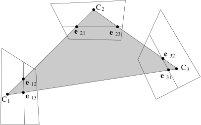
Denoting the cameras by 1,2,3, there are now three fundamental matrices, F1,2, F1,3, F2,3, and six epipoles, ei,j, as in Figure 11. The three fundamental matrices describe completely the trifocal geometry (Faugeras and Robert,1994).

The plane containing the three optical centres is called the trifocal plane. It intersects each image plane along a line which contains the two epipoles.

Writing Eq. (45) for each camera pair (taking the centre of the third camera as the point M) results in three epipolar constraints:

F3,1⁢e3,2≃e1,3⁢e1,2⁢F1,2⁢e1,3≃e2,1⁢e2,3⁢F2,3⁢e2,1≃e3,2×e3,1

(64)

Three fundamental matrices include 21 free parameters, less the 3 constraints above; the trifocal geometry is therefore determined by 18 parameters.

This description of the trifocal geometry fails when the three cameras are collinear, and the trifocal plane reduces to a line.

§ 5.1.1. Point transfer

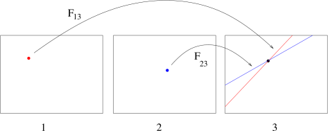
Figure 12. Point transfer using epipolar constraints between three views.

If the trifocal geometry is known, given two conjugate points m1 and m2 in view 1 and 2 respectively, the position of the conjugate point m3 in view 3 is completely determined (Figure 12).

This allows for point transfer or prediction. Indeed, m3 belongs simultaneously to the epipolar line of m1 and to the epipolar line of m2, hence:

m3≃F1,3⁢m1⁢F2,3⁢m2

(65)

View synthesisLaveau and Faugeras (1994); Avidan and Shashua (1997); Boufama (2000), exploit the trifocal geometry to generate novel (synthetic) images starting from two reference views. A related topic is image-based rendering(Lengyel,1998; Zhang and Chen,2003; Isgrò et al.,2004).

Epipolar transfer fails when the three optical rays are coplanar, because the epipolar lines are coincident. This happens:

if the 3-D point is on the trifocal plane;
if the three cameras centres are collinear (independently of the position of 3-D point).

These deficiencies motivate the introduction of an independent trifocal constraint.

In addition, by generalizing the case of two views, one might conjecture that the trifocal geometry should be represented by a trilinear form in the coordinates of three conjugate points.

§ 5.2. The trifocal constraint

Consider a point M in space projecting to m1, m2 and m3 in three cameras

P1=[I|0],P2=[A2|e2,1],andP3=[A3|e3,1].

(66)

Let us write the epipolar line of m1 in the other two views (using Eq. (23)):

	ζ2⁢m2	=e2,1+ζ1⁢A2⁢m1		(67)
	ζ3⁢m3	=e3,1+ζ1⁢A3⁢m1.		(68)

where ζi varies in R and correspond to the depth of the 3D point with respect to view i.

Consider a line through m2, represented by s2; we have s2T⁢m2=0, that substituted in (67) gives:

0=s2T⁢e2,1+ζ1⁢s2T⁢A2⁢m1

(69)

Likewise, for a line through m3 represented by s3 we can write:

0=s3T⁢e3,1+ζ1⁢s3T⁢A3⁢m1

(70)

After eliminating ζ1 from Equation (69) and (70) we obtain:

0=s2T⁢e2,1⁢s3T⁢A3⁢m1-s3T⁢e3,1⁢s2T⁢A2⁢m1

(71)

and after some re-writing:

0=s2T⁢e2,1⁢m1T⁢A3T-A2⁢m1⁢e3,1T⁢s3

(72)

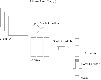
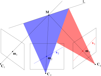
This is the trifocal constraint, that links (via a trilinear form) m1, s2 (any line through m2) and s3 (any line through m3).

Geometrically, the trifocal constraint imposes that the optical rays of m1 intersect the 3-D line L that projects onto s2 in the second image and s3 in the third image.

Please note that given two (arbitrary) lines in two images, they can be always seen as the image of a 3-D line L, because two planes always define a line, in projective space (this is why there is no such thing as the epipolar constraint between lines.)

The trifocal constraint represents the trifocal geometry (nearly) without singularities. It only fails is when the cameras are collinear and the 3-D point is on the same line.

Figure 13. Two arbitrary lines s2 and s3 through corresponding points m2 and m3 in the second and third image respectively, define a 3-D line L that must intersect the optical ray of m1.

Using the properties of the Kronecker product, the trifocal constraint (Eq. (72)) can be written as:

0	=s3T⊗s2T⁢v⁢e⁢c⁢e2,1⁢m1T⁢A3T-A2⁢m1⁢e3,1T
	=s3T⊗s2T⁢A3⊗e2,1⁢v⁢e⁢c⁢m1-e3,1⊗A2⁢v⁢e⁢c⁢m1
	=(s3T⊗s2T)((A3⊗e2,1)-(e3,1⊗A2))m1)
	=s3T⊗s2T⁢T⁢m1	(73)

where T is the 9×3 trifocal matrix (Fusiello,) defined by

T=A3⊗e2,1-e3,1⊗A2

(74)

The matrix T encodes the trifocal geometry. Its 27 entries are the coefficient of the trilinear form.

An equivalent formulation of the trifocal constraint that generalizes the expression of a bilinear form (Cfr. pg. 4.5.2) is obtained by applying once again the property v⁢e⁢c⁢A⁢X⁢B=BT⊗A⁢v⁢e⁢c⁢X:

m1T⊗s3T⊗s2T⁢v⁢e⁢c⁢T=0.

(75)

§ 5.2.1. Trifocal constraint for lines.

Consider a line L in space projecting to s1, s2 and s3 in the three cameras. The trifocal constraint must hold for any point m1 contained in the line s1:

s3T⊗s2T⁢T⁢m1=0⁢∀m1:s1T⁢m1=0

(76)

hence

s1T=s3T⊗s2T⁢T

(77)

This is the trifocal constraint for lines, which also allows direct line transfer: if s3 and s2 are two lines in the third and second view respectively, the image s1 in the first view of the line in space determined by s2 and s3 is obtained by means of the trifocal matrix.

§ 5.2.2. Trifocal constraints for points.

In Eq. (72), s2 is any line through m2, and s3 is any line through m3.
Each row of m2× (resp. m3×) represents a line through m2 (resp. m3), because m2×⁢m2=0.

Hence we can write a total of nine constraints similar to Eq. (72), only four of which are independent (two for each point):

m2×⁢e2,1⁢m1T⁢A3T-A2⁢m1⁢e3,1T⁢m3×=03×3.

(78)

Hence, the trifocal constraints for three points writes:

m3×⊗m2×⁢T⁢m1=0.

(79)

Or, equivalently

m1T⊗m3×⊗m2×⁢v⁢e⁢c⁢T=0

(80)

This equation can be used to recover T (likewise we did for F). The coefficient matrix is a 9×27 matrix; its rank is four, being the Kronecker product of a vector by a rank-2 matrix by a rank-2 matrix.

Therefore, every triplet {m1, m2, m3} of corresponding points gives four linear independent equations. Seven triplets determine the 27 entries of T.

§ 5.2.3. Point transfer.

A third equivalent formulation of the trifocal constraint is derived if we look at the vector T⁢m1 in Eq. (73) as the vectorization of a suitable matrix. This is easy to write thanks to the vector transposition²

The vector transposition operator Apgeneralizes the transpose of a matrix A by operating on vectors of p entries at a time.

0	=s3T⊗s2T⁢T⁢m1
	=s3T⊗s2T⁢v⁢e⁢c⁢T⁢m13
	=s2T⁢T⁢m13⁢s3	(81)

where T⁢m13 is a 3×3 matrix such that v⁢e⁢c⁢T⁢m13=T⁢m1.

By the same token as before, one can stack three equations similar to Eq. (81) as:

s2T⁢T⁢m13⁢m3×=0

(82)

This implies that the transpose of the leftmost term in parentheses (which is a 3-D vector) belongs to the kernel of m3×, which is equal to m3 (up to a scale factor) by construction. Hence

m3≃T⁢m13T⁢s2

(83)

This is the point transfer equation: if m1 and m2 are conjugate points in the first and second view respectively, the position of the conjugate point m3 in the third view is computed by means of the trifocal matrix.

§ 5.2.4. Homography from the trifocal matrix

A line s2 in the second view defines (by back-projection) a 3-D plane, which induces a homography H between the first and the third view.

Hence, s3=HT⁢s1 since s1 and s3 are both projection of the same line, that belongs to the plane ³

The reader can verify that if H is the homography induced by a plane between two views, such that conjugate points are related by m2=H⁢m1, conjugate lines are related by s2=HT⁢s1.

On the other hand, Eq. (77) is equivalent to

s1=I3×3⊗s2T⁢T3⁢s3.

Hence, the homography H can be expressed in terms of the trifocal matrix as:

HT=I3×3⊗s2T⁢T3

§ 5.2.5. Relationship with the trifocal tensor.

The Kronecker notation and the tensorial notation are deeply related, as both represents multilinear forms. To draw this relationship in the case of the trifocal geometry, let us expand the trifocal matrix into its columns T=t1⁢t2⁢t3 and m1 into its components m1=u,v,wT. Then, thanks to the linearity of the vector transposition:

T⁢m13=t1⁢t2⁢t3⁢m13=u⁢t1+v⁢t2+w⁢t33=u⁢t13+v⁢t23+w⁢t33

(84)

This implies that T⁢m13 can be seen as the linear combination of the matrices t13,t23,t33 with the components of m1 as coefficients. Therefore, the action of the trilinear form Eq. (81) is to first combine matrices t13,t23,t33 according to m1, then combine the columns of the resulting matrix according to s3 and finally to combine the elements of the resulting vector according to s2, to obtain a scalar.

The 3×3×3 array T obtained by stacking the three 3×3 matrices t13,t23,t33 is the trifocal tensor.

Figure 14. Action of a trilinear form f(a,b,c) represented by a tensor.

§ 5.3. Reconstruction

As in the case of two views, what can be reconstructed depends on what is known about the scene and the cameras.

If the intrinsic parameters of the cameras are known, we can obtain a Euclidean reconstruction, that differs from the true reconstruction by a similarity transformation. This is composed by a rigid displacement (due to the arbitrary choice of the world reference frame) plus a a uniform change of scale (due to the well-known depth-speed ambiguity).

In the weakly calibrated case, i.e., when point correspondences are the only information available, a projective reconstruction can be obtained.

In both cases, the solution is not a straightforward generalization of the two view case, as the problem of global consistency comes into play (i.e., how to relate each other the local reconstructions that can be obtained from view pairs).

§ 5.3.1. Euclidean Reconstruction

Let us consider for simplicity the case of three views, which generalizes straightforward to N views.

If one applies the method of Section 4.4.2 to view pairs 1-2, 1-3 and 2-3 one obtains three displacements R12,t⌃12,R13,t⌃13 and R23,t⌃23 known up a scale factor, as the norm of translation cannot be recovered, (the symbol ⌃ indicates a unit vector).

The “true” displacements must satisfy the following compositional rule

t13=R23⁢t12+t23

(85)

which can be rewritten as

t⌃13=μ1⁢R23⁢t⌃12+μ2⁢t⌃23

(86)

where μ1=t12/t13 and μ2=t23/t13 are unknown.

However, Eq. (85) constraints t⌃13,R23⁢t⌃12 and t⌃23 to be coplanar, hence the ratios μ1,μ2 can be recovered:

t12t13=μ1=t⌃13×t⌃23⋅R23×t⌃12×t⌃23R23×t⌃12×t⌃232

(87)

And similarly for μ2.

In this way three consistent camera matrices can be instantiated.

Note that only ratios of translation norm can be computed, hence the global scale factor remains undetermined.

§ 5.3.2. Projective Reconstruction

If one applies the method of Section 4.5.3 to consecutive pairs of views, she would obtain, in general, a set of reconstructions linked to each other by an unknown projective transformation (because each camera pair defines its own projective frame).

The trifocal geometry could be used to link together consistently triplets of views. In Section 4.5.3 we saw how a camera pair can be extracted from the fundamental matrix. Likewise, a triplet of consistent cameras can extracted from the trifocal matrix (or tensor). The procedure is more tricky, though.

An elegant method for multi-image reconstruction was described in Sturm and Triggs (1996), based on the same idea of the factorization method of Tomasi and Kanade (1992).

Consider m cameras P1⁢…⁢Pm looking at n 3-D points M1⁢…⁢Mn. The usual projection equation

ζij⁢mij=Pi⁢Mj⁢i=1⁢…⁢m,j=1⁢…⁢n.

(88)

can be written in matrix form:

ζ11⁢m11ζ12⁢m12…ζ1n⁢m1nζ21⁢m21ζ22⁢m22…ζ2n⁢m2n⋮⋮⋱⋮ζm1⁢mm1ζm2⁢mm2…ζmn⁢mmn︸scaled measurements ⁢W=P1P2⋮Pm︸P⁢M1,M2,…Mn︸structure ⁢M.

(89)

In this formula the mij are known, but all the other quantities are unknown, including the projective depths ζij. Equation (89) tells us that W can be factored into the product of a 3×m×4 matrix P and a 4×n matrix M. This also means that W has rank four.

If we assume for a moment that the projective depths ζij are known, then matrix W is known too and we can compute its singular value decomposition:

W=U⁢D⁢VT.

(90)

In the noise-free case, D=diag⁢σ1,σ2,σ3,σ4,0,…⁢0, thus, only the first 4 columns of U (V) contribute to this matrix product. Let U3×m×4 (Vn×4) the matrix of the first 4 columns of U (V). Then:

W=U3×m×4⁢diag⁢σ1,σ2,σ3,σ4⁢Vn×4T.

(91)

The sought reconstruction is obtained by setting:

P=U3×m×4⁢diag⁢σ1,σ2,σ3,σ4⁢and⁢M=Vn×4T

(92)

This reconstruction is unique up to a (unknown) projective transformation. Indeed, for any non singular projective transformation T, T⁢P and T-1⁢M is an equally valid factorization of the data into projective motion and structure.

Consistently, the choice to subsume diag⁢σ1,σ2,σ3,σ4 in P is arbitrary.

In presence of noise, σ5 will not be zero. By forcing D=diag⁢σ1,σ2,σ3,σ4,0,…⁢0 one computes the solution that minimizes the following error:

W-P⁢MF2=∑i,jζij⁢mij-Pi⁢Mj2

where ||⋅||F is the Frobenius norm.

As the depth ζij are unknown, we are left with the problem of estimating them.

An iterative solution is to alternate estimating ζij (given P and M) with estimating P and M (givenζij).

If P and M are known, estimating ζij is a linear problem. Indeed, for a given point j the projection equation writes:

ζ1j⁢m1jζ2j⁢m2j⋮ζmj⁢mmj=m1j0…00m2j…0⋮⋮⋱⋮00…mmj︸Qj⁢ζ1jζ2j⋮ζmj︸ζj=P⁢Mj

(93)

Starting from an initial guess for ζij (typically ζij=1), the following iterative procedure⁴

Whilst this procedure captures the main idea of Sturm and Triggs, it is not exactly the algorithm proposed in (Sturm and Triggs,1996). To start with, the original algorithm (Sturm and Triggs,1996) was not iterative and used the epipolar constraint (Eq.45) to fix the ratio of the projective depths of one point in successive images. It was Triggs (1996) who made the scheme iterative. Moreover in (Sturm and Triggs,1996) the normalization of W is performed by normalizing rows and columns of W. The Frobenius norm was used by (Oliensis,1999). A similar scheme was also proposed by Heyden (1997).

is used:

Normalize W such that WF=1;
Factorize W and obtain an estimate of P and M;
If W-P⁢MF2 is sufficiently small then stop;
Solve for ζj in Qj⁢ζj=P⁢Mj, for all j=1⁢…⁢n;
Update W.
Goto 1.

Step 1 is necessary to avoid trivial solutions (e.g. ζij=0).

This technique is fast, requires no initialization, and gives good results in practice, although there is no guarantee that the iterative process will converge. A provably convergent iterative method has been presented by Mahamud et al. (2001).

§ 5.4. Multifocal constraints

We outline here an alternative and elegant way to derive all the meaningful multi-linear constraints on N views, based on determinants, described in (Heyden,1998). Consider one image point viewed by m cameras:

ζi⁢mi=Pi⁢M⁢i=1⁢…⁢m

(94)

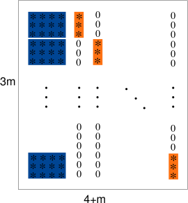
By stacking all these equations we obtain:

P1m10…0P20m2…0⋮⋮⋮⋱⋮Pm00…mm︸L⁢M-ζ1-ζ2⋮-ζm=00⋮

(95)

This implies that the 3×m×m+4 matrix L is rank-deficient, i.e., r⁢a⁢n⁢k⁢L<m+4. In other words, all the m+4×m+4 minors of L are equal to 0.

The minors that does not contain at least one row from each camera are identically zero, since they contain a zero column.

If a minor contains only one row from some view, the image coordinate corresponding to this row can be factored out (using Laplace expansion along the corresponding column).

Hence, at least one row has to be taken from each view to obtain a meaningful constraint, plus another row from each camera to prevent the constraint to be trivially factorized.

Figure 15. Visualization of the structure of the matrix L.

Since there are m views, after taking one row from each camera, the remaining four rows can be chosen as follows:

Two rows from one view and two rows from another view.
Two rows from one view, one row from another view and one row from a third view.
One row from each of four different views.

If m=2 choosing two rows from one view and two rows from another view gives a bilinear two-view constraint, expressed by the bifocal tensor i.e., the fundamental matrix.

If m=3, choosing two rows from one view, one row from another view and one row from a third view gives a trilinear three-view constraint, expressed by the trifocal tensor.

If m=4, choosing one row from each of four different views gives a quadrilinear four-view constraint, expressed by the quadrifocal tensor.

If m>4, there is no way to avoid that the minors contain only one row from some views. Hence, constraints involving more than 4 cameras can be factorised as product of the two-, three-, or four-views constraints and image point coordinates.

This indicates that no interesting constraints can be written for more than four views⁵

Actually, it can be proven that also the quadrifocal constraints are not independent (Ma et al.,2003).

Please note that Eq. (95) can be also used to triangulate one point M in multiple views, by solving the homogeneous linear system for M,-ζ1,-ζ2,⋯,-ζmT.