§ 7. Getting practical
In this section we will approach estimation problems from a more “practical” point of view.
First, we will discuss how the presence of errors in the data affects our estimates and describe the countermeasures that must be taken to obtain a good estimate.
Second, we will introduce non-linear distortions due to lenses into the pinhole model and we illustrate a practical calibration algorithm that works with a simple planar object.
Finally, we will describe rectification, a transformation of image pairs such that conjugate epipolar lines become collinear and parallel to one of the image axes, usually the horizontal one. In such a way, the correspondence search is reduced to a 1D search along the trivially identified scanline.
§ 7.1. Pre-conditioning
In presence of noise (or errors) on input data, the accuracy of the solution of a linear system depends crucially on the condition number of the system. The lower the condition number, the less the input error gets amplified (the system is more stable).
As Hartley (1995) pointed out, it is crucial for linear algorithms (as
the DLT algorithm) that input data is properly pre-conditioned, by a
suitable coordinate change (origin and scale): points are translated
so that their centroid is at the origin and are scaled so that their
average distance from the origin is
This improves the condition number of the linear system that is being solved.
Apart from improved accuracy, this procedure also provides invariance under similarity transformations in the image plane.
§ 7.2. Algebraic vs geometric error
Measured data (i.e., image or world point positions) is noisy.
Usually, to counteract the effect of noise, we use more equations than necessary and solve with least-squares.
What is actually being minimized by least squares?
In a typical null-space problem formulation
In general, if
All the linear algorithm (DLT and others) we have seen so far minimize an algebraic error. Actually, there is no justification in minimizing an algebraic error apart from the ease of implementation, as it results in a linear problem.
Usually, the minimization of a geometric error is a non-linear problem, that admit only iterative solutions and requires a starting point.
So, why should we prefer to minimize a geometric error? Because:
-
The quantity being minimized has a meaning
-
The solution is more stable
-
The solution is invariant under Euclidean transforms
Often linear solution based on algebraic residuals are used as a starting point for a non-linear minimization of a geometric cost function, which “gives the solution a final polish” (Hartley and Zisserman,2003).
§ 7.2.1. Geometric error for resection
The goal is to estimate the camera matrix, given a number of
correspondences
The geometric error associated to a camera estimate
| (116) |
where
The DLT solution is used as a starting point for the iterative minimization (e.g. Gauss-Newton)
§ 7.2.2. Geometric error for triangulation
The goal is to estimate the 3-D coordinates of a point
The geometric error associated to a point estimate
| (117) |
where
The linear solution is used as a starting point for the iterative minimization (e.g. Gauss-Newton).
§ 7.2.3. Geometric error for F
The goal is to estimate
The geometric error associated to an estimate
| (118) |
where
The eight-point solution is used as a starting point for the iterative minimization (e.g. Gauss-Newton).
Note that
§ 7.2.4. Geometric error for H
The goal is to estimate
The geometric error associated to an estimate
| (119) |
where
The linear solution is used as a starting point for the iterative minimization (e.g. Gauss-Newton).
§ 7.2.5. Bundle adjustment (reconstruction)
If measurements are noisy, the projection equation will not be satisfied exactly by the camera matrices and structure computed in Sec. 5.3.2.
We wish to minimize the image distance between the re-projected point
| (120) |
where
As
A solution is to alternate minimizing the re-projection error by
varying
See (Triggs et al.,2000) for a review and a more detailed discussion on bundle adjustment.
§ 7.3. Robust estimation
Up to this point, we have assumed that the only source of error affecting correspondences is in the measurements of point's position. This is a small-scale noise that gets averaged out with least-squares.
In practice, we can be presented with mismatched points, which are outliers to the noise distribution (i.e., rogue measurements following a different, unmodelled, distribution).
These outliers can severely disturb least-squares estimation (even a single outlier can totally offset the least-squares estimation, as illustrated in Fig. 16.)
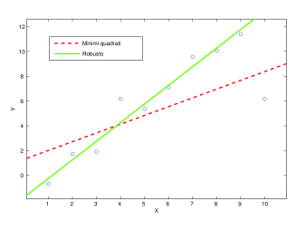
The goal of robust estimation is to be insensitive to outliers (or at least to reduce sensitivity).
§ 7.3.1. M-estimators
Least squares:
| (121) |
where
| (122) |
Differentiating with respect to
| (123) |
The M-estimate is obtained by solving this system of non-linear equations.
§ 7.3.2. RANSAC
Given a model that requires a minimum of
-
Randomly select a subset of
-
Determine the set
-
If the size of
-
If the size of
-
Terminate after
Three parameters need to be specified:
Both
| (124) |
By requiring that
At each iteration, the largest consensus set found so fare gives a
lower bound on the fraction of inliers, or, equivalently, an upper
bound on the number of outliers. This can be used to adaptively adjust
the number of trials
As pointed out by Stewart (1999), RANSAC can be viewed as a particular M-estimator.
The objective function that RANSAC maximizes is the number of data
points having absolute residuals smaller that a predefined value
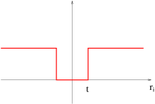
By virtue of the prespecified inlier band, RANSAC can fit a model to data corrupted by substantially more than half outliers.
§ 7.3.3. LMedS
Another popular robust estimator is the Least Median of Squares. It is defined by:
| (125) |
It can tolerate up to 50% of outliers, as up to half of the data point can be arbitrarily far from the “true” estimate without changing the objective function value.
Since the median is not differentiable, a random sampling strategy
similar to RANSAC is adopted. Instead of using the consensus, each
sample of size
A final weighted least-squares fitting is used.
With respect to RANSAC, LMedS can tolerate “only” 50% of outliers, but requires no setting of thresholds.
§ 7.4. Practical calibration
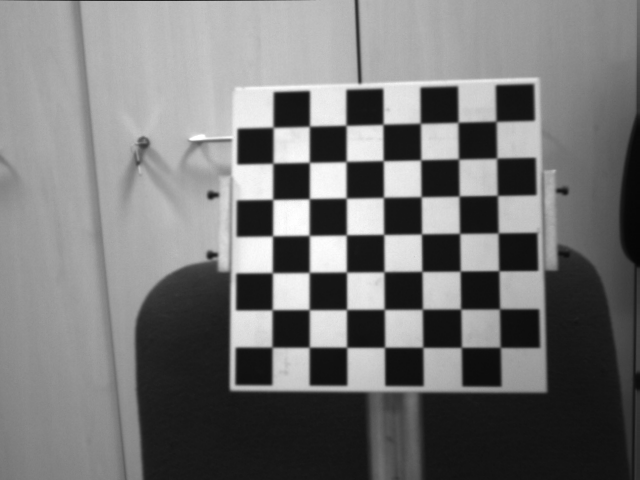
Camera calibration (or resection) as described so far, requires a calibration object that consists typically of two or three planes orthogonal to each other. This might be difficult to obtain, without access to a machine tool.
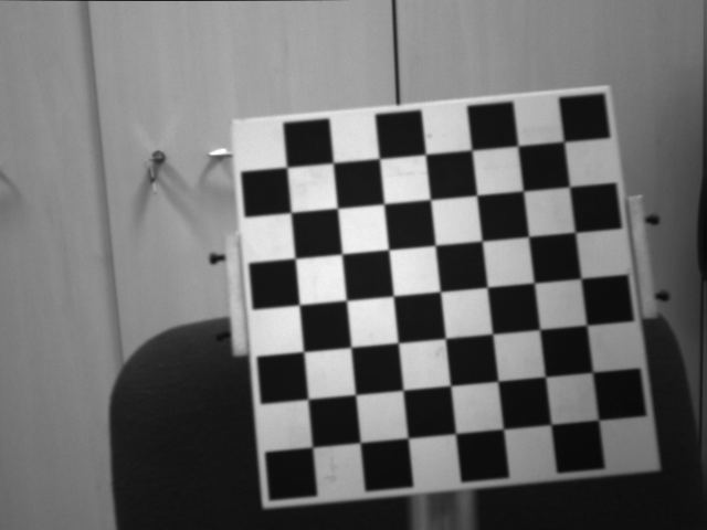
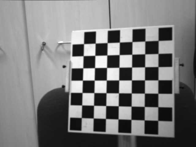
Zhang (1998) introduced a calibration technique that requires the camera to observe a planar pattern (much easier to obtain) at a few (at least three) different orientation. Either the camera or the planar pattern can be moved by hand.
Instead of requiring one image of many planes, this method requires many images of one plane.
We will also introduce here a more realistic camera model that takes into account non-linear effects produced by lenses.
In each view, we assume that correspondences between image points and 3-D points on the planar pattern have been established.
§ 7.4.1. Estimating intrinsic parameters
Following the development of Sec. 4.6 we know that for a camera
| (126) |
where
Suppose that
Writing
| (127) |
where
The orthogonality
| (128) |
or, equivalently
(remember that
| (129) |
Likewise, the condition on the norm
| (130) |
Introducing the Kronecker product as usual, we rewrite these two equations as:
| (131) | |||
| (132) |
As
| (133) | |||
| (134) |
From a set of
At least five equations are needed (
§ 7.4.2. Estimating extrinsic parameters
| (135) |
Because of noise, the matrix
Let
In this way we have obtained the camera matrix
It is advisable to refine it with a (non-linear) minimization of a geometric error:
| (136) |
where
The linear solution is used as a starting point for the iterative minimization (e.g. Gauss-Newton).
§ 7.4.3. Radial distortion
A realistic model for a photocamera or a videocamera must take into account non-linear distortions introduced by the lenses, especially when dealing with short focal lengths or low cost devices (e.g. webcams, disposable cameras).
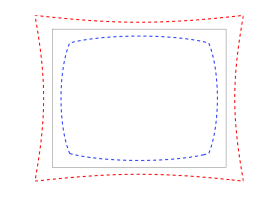
The more relevant effect is the radial distortion, which is
modeled as a non-linear transformation from the ideal (undistorted)
pixel coordinates
| (137) |
where
This distortion makes a rectangle to appear as a “barrel” or a “cushion” (as
in Fig. 19) depending whether the coefficient
§ 7.4.4. Estimating k 1
Let us assume that the pinhole model is calibrated. The point
We wish to recover
| (138) |
hence a least squares solution for
When calibrating a camera we are required to simultaneously estimate both the pinhole model's parameters and the radial distortion coefficient.
The pinhole calibration we have described so far assumed no radial distortion, and the radial distortion calibration assumed a calibrated pinhole camera.
The solution (a very common one in similar cases) is to alternate between the two estimation until convergence.
Namely: start assuming
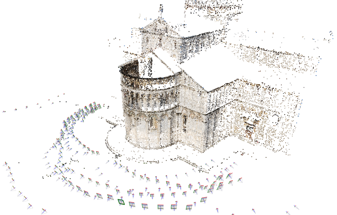
§ 7.5. Practical multi-view reconstruction
The multi-view projective reconstruction method based on factorization, albeit elegant, is of little practical use, because it assumes that all the point are visible in all the views. The method for Euclidean reconstruction, based on the factorization of essential matrices is more effective, but it does not scale well with large scale scenarios. The best results in the state of the art have been demonstrated by pipelines based on the idea of growing partial reconstructions, composed by cameras and points, where new cameras are added by resection and new points by intersection. Frequent bundle adjustments avoid drift. Some examples of such pipelines are (Brown and Lowe,2005; Kamberov et al.,2006; Snavely et al.,2006; Vergauwen and Gool,2006; Irschara et al.,2007), and (Gherardi et al.,2010). An example of the latter is shown in Fig. 20.