Tutorial #A07: Lidar data management and integration
Welcome to the 3DF Zephyr tutorial series.
The following tutorial will focus on how to deal with LiDAR data in 3DF Zephyr, including laser scan registration and integration between LiDAR and photogrammetry data.
This tutorial cannot be completed with 3DF Zephyr Free or 3DF Zephyr Lite!
Summary
Introduction
Registration is the process of aligning two or more scans, either done based on a reference scan or using common reference positions between scans to create the most accurate alignment possible.
This tutorial has three sections:
- Section A: LiDAR data registration
Learn how to import and register laser scans in 3DF Zephyr.
- Section B: Automatic register images to scans
Learn how to orient images starting from a group of laser scans.
- Section C: LiDAR and photogrammetry data integration
This section will guide you through integrating LiDAR and photogrammetry data in 3DF Zephyr.
Section A: LiDAR data registration
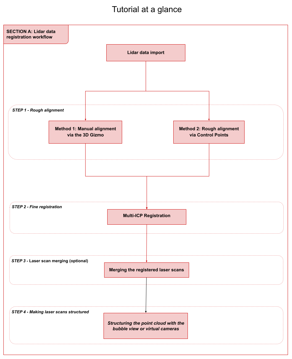
LiDAR data import
This first tutorial’s part explains how to import and prepare the laser scans inside 3DF Zephyr before the other phases.
Zephyr allows for importing the following laser-scanning file formats:
-
– Common file formats: .ply, .pts, .ptx, .las, .e57, .xyz, .txt, .rcp, .laz;
– Native file formats: .fls (Faro), .fws (Faro), .rdb (Riegl), .rdbx (Riegl), .zfs ( Z+F), Stonex, .dp (Dot product), .x3a (Stonex);
Note: Native scan file formats require importing specific plug-ins in 3DF Zephyr. Please, download and install the necessary plug-ins before starting the tutorial, following this link: https://www.3dflow.net/native-laser-scanner-support-plugin-3df-zephyr-download/
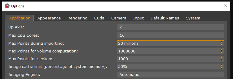
Before importing the scans, you can decrease/increase the number of points during the import process; based on this value, 3DF Zephyr will perform a point decimation in the scans.
Click the Options > Application tab and change the option Maximum number of points during importing (default value: 30 million).
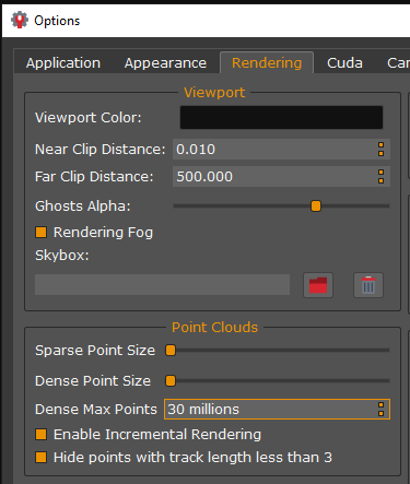
In addition, the maximum visible points number can be set to reduce/increase the number of visible points in the workspace. 3DF Zephyr will perform only a visual decimation, preserving the actual number of imported points.
Click Options > Rendering tab; in the Point Clouds section, change the value of the Dense max points (default value: 30 million ).
Open a new software session and drag and drop your laser scan files into the workspace. Alternatively, you can click the Import menu, select the Import model option and then select the files you want to import inside 3DF Zephyr.
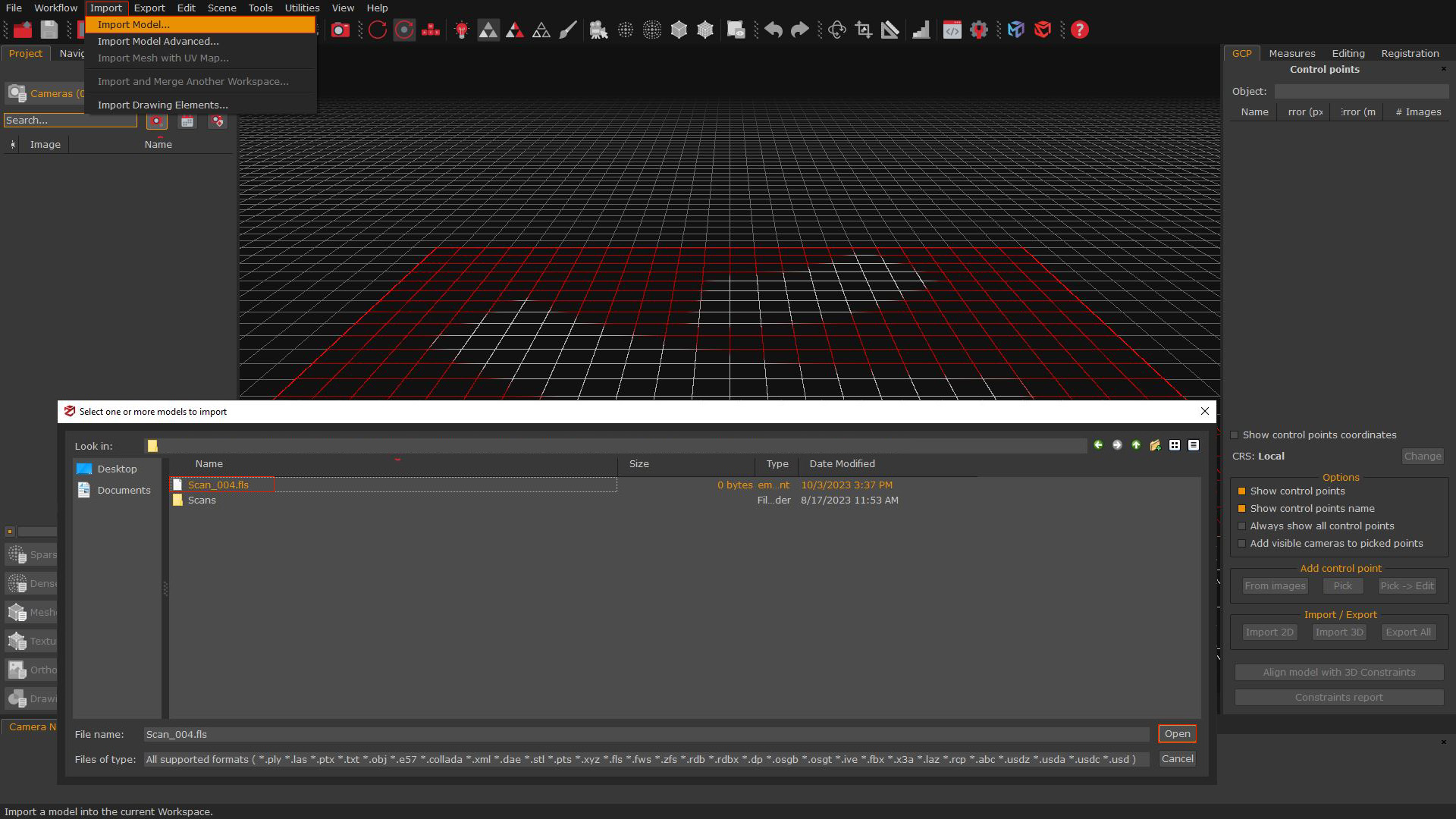
In the both method, for importing additional scans, it is recommended to directly drag or import the scan file (e.g., .fls) into the workspace, rather than importing the entire folder.
When utilizing the drag and drop method, please ensure to click the “Merge” button for confirmation of the import process.
STEP 1 – Rough alignment
You can pick either Method 1 or 2, described below, to align your LiDAR data roughly.
Method 1: Manual alignment via the 3D Gizmo
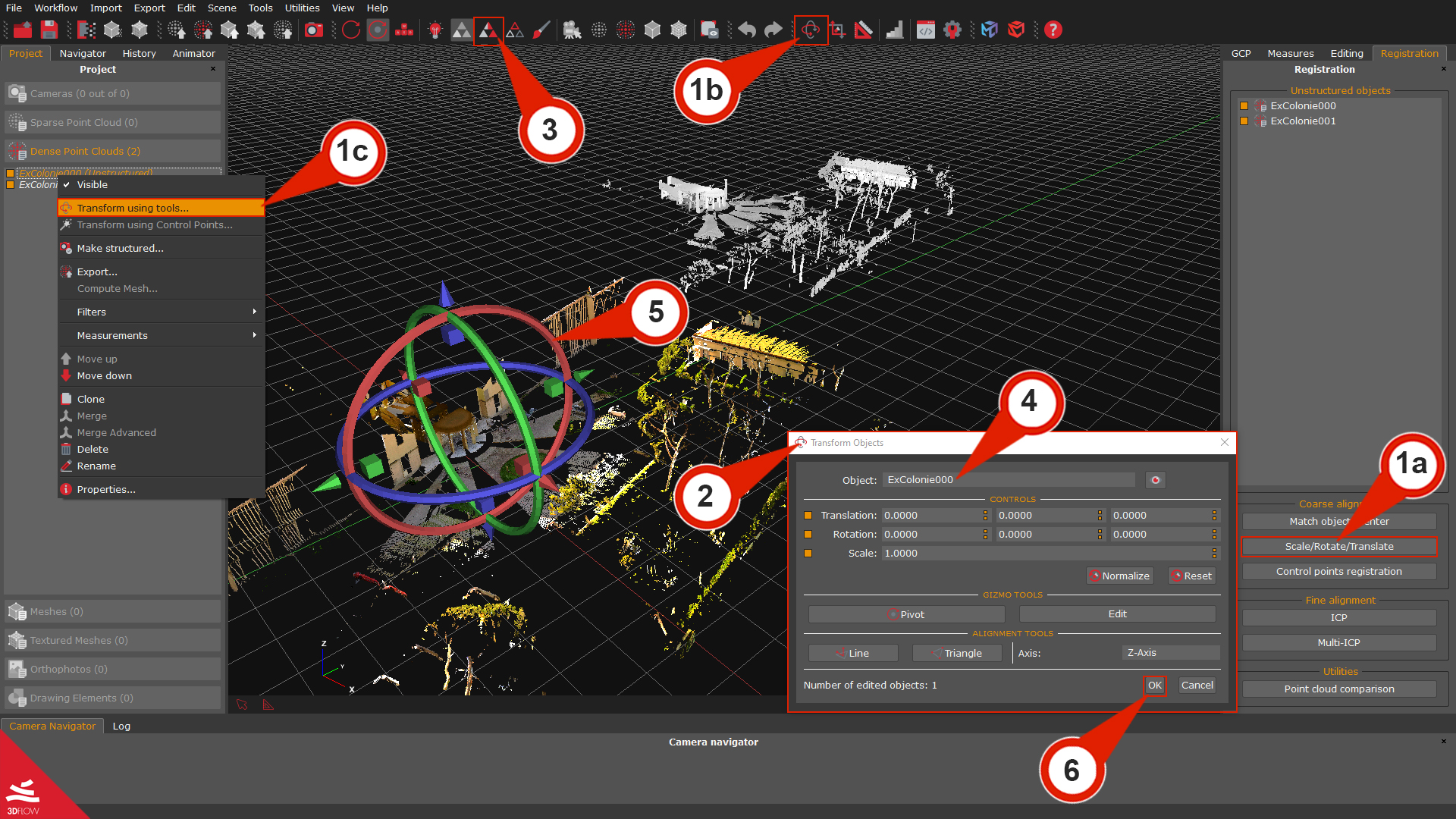
You can use the Gizmo to bring the scans to a rough alignment. You can enable the “Gizmo tool” by:
– Using the Registration tab on the right side of the user interface (click the “Scale/rotate/translate” (1a) button.).
– Clicking the “Scale/rotate/translate objects (1b)” button in the top toolbar.
– Right-clicking the target scan and selecting the “Transform using tools” (1c) option.
The “Transform object” (2) window will appear.
When using the 3D gizmo, please notice that it’s better to enable the visualization of all the desired items using their related checkbox in the Project tab before starting the rough alignment. To ease the alignment visualization, you can also enable the “Uniform colors” (3) view by clicking the related button in the toolbar.
From the dropdown box “Object” (4), you can also select which scan will be moved using the 3D gizmo (5).
Once You have aligned a couple of scans, click the “OK” (6) button before exiting the gizmo tool to confirm the roto translation.
Method 2: Rough alignment via control points
This rough alignment method will be performed using placed control points on the scans.
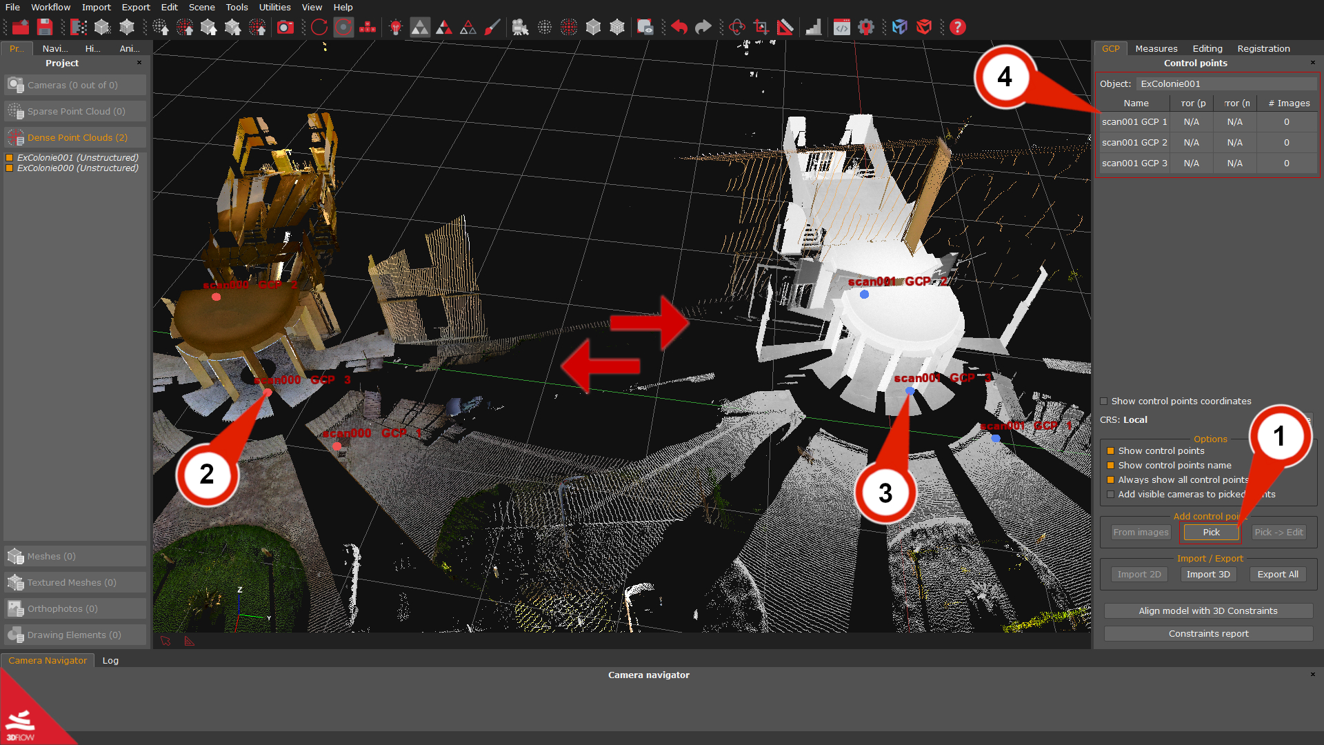
Click the “Pick”(1) button in the GCP panel and place a minimum of three control points on the first scan (2). Afterward, you must apply the same control points positions (3) over the other scan (six control points at all).
Note: Please, make sure to place the control points on the same areas that you will be able to recognize easily on both laser scans. Usually, edges work very well. Keep in mind that it is better to select points that are located on all three axes.
The added control points will be listed in the GCP panel (4) depending on their reference object.
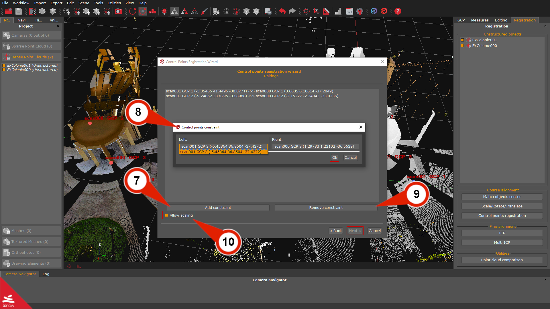
Once done, select the “Control point registration” (5) button in the Registration tab. The Control point registration wizard (6) will appear.
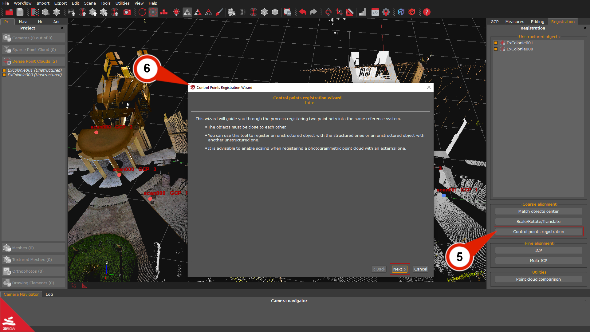
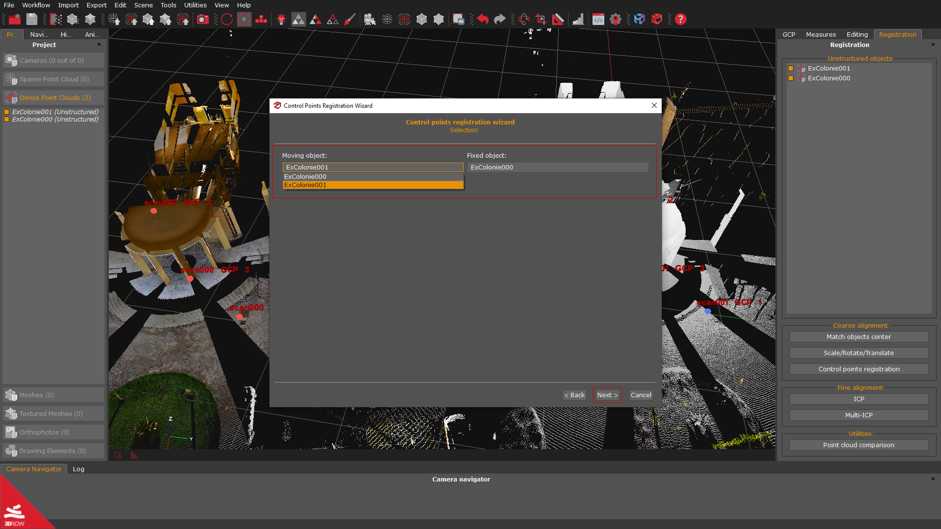
Click the “Next” button on the second page; you can select which object will be the “Moving Object” and which one will be the “Fixed Object”. Click on the “Next” button.
On the Parings page, use the “Add Constraint” (7) button to select the pairings (8) accordingly to the control points labels that you have previously used; at least three couples of control points are required. It is also possible to remove the pairing using the “Remove constraint” (9) button, and before proceeding, it is also recommended to check the Allow scaling (10) checkbox.
Click the “Next” button and the “Apply” button on the next page to start the rough alignment. You can repeat the process for all the scans that need a rough alignment before the fine registration step.
Step 2 – Fine Registration
Once the Rough alignment with the 3D Gizmo or the Control points has been completed, you can leverage the ICP (Iterative closest point) algorithm to minimize the point distance between the scans. While the ICP option allows the algorithm to deal with two elements, the Multi-ICP algorithm allows dealing with more than two laser scans.
Please remember that:
-
– the objects must be close to each other;
– the adjustment and the minimization will be performed globally;
– if you need to register point sets with different scales, it is advisable to use the two-view ICP dialog and enable scaling.
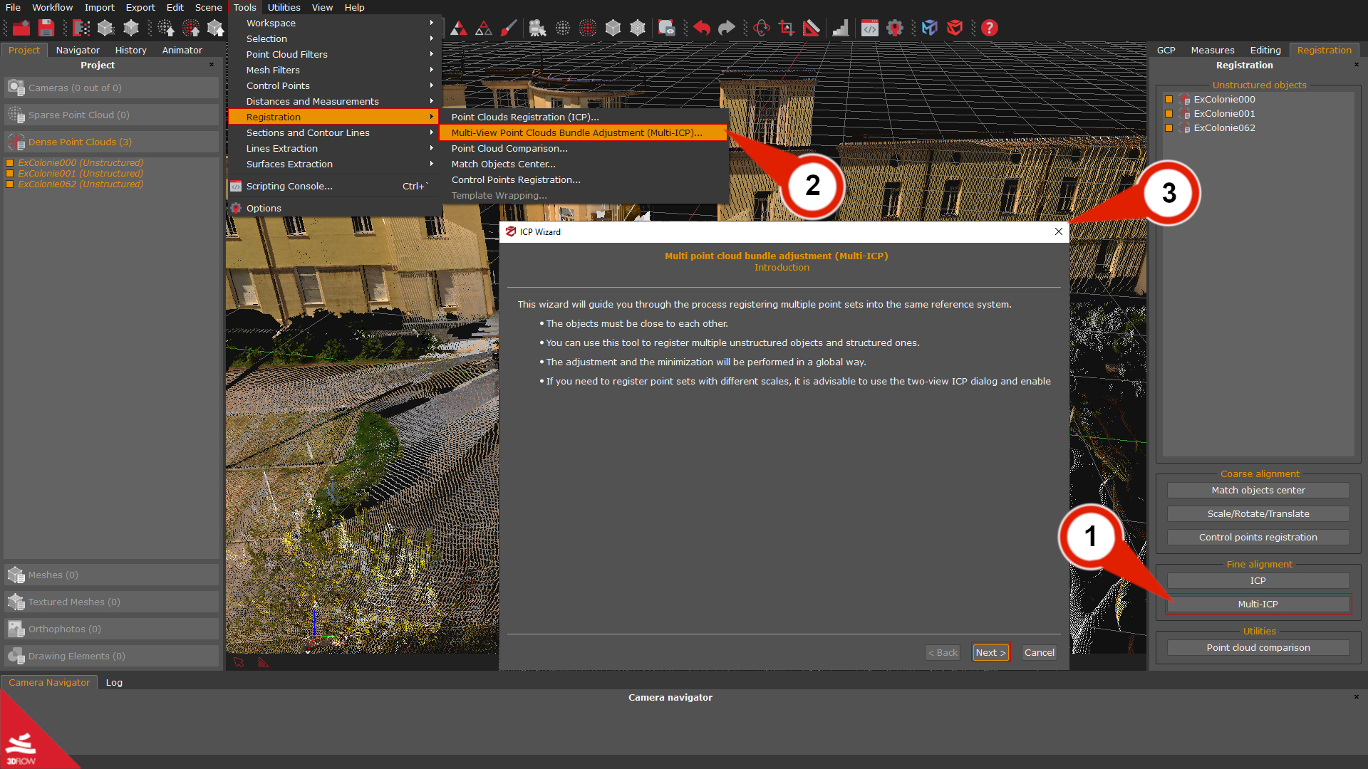
Click on the “Multi-ICP” (1) button in the Registration tab on the right side of the workspace, or alternatively is possible to go to the menu Tools > Registration > Multi view point cloud bundle adjustment (2) for opening the Multi-ICP Wizard (3).
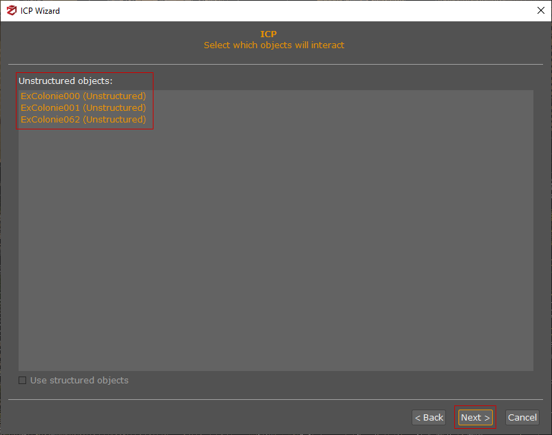
In the Select which object will interact page, select the scans you want to align and click the “Next” button.
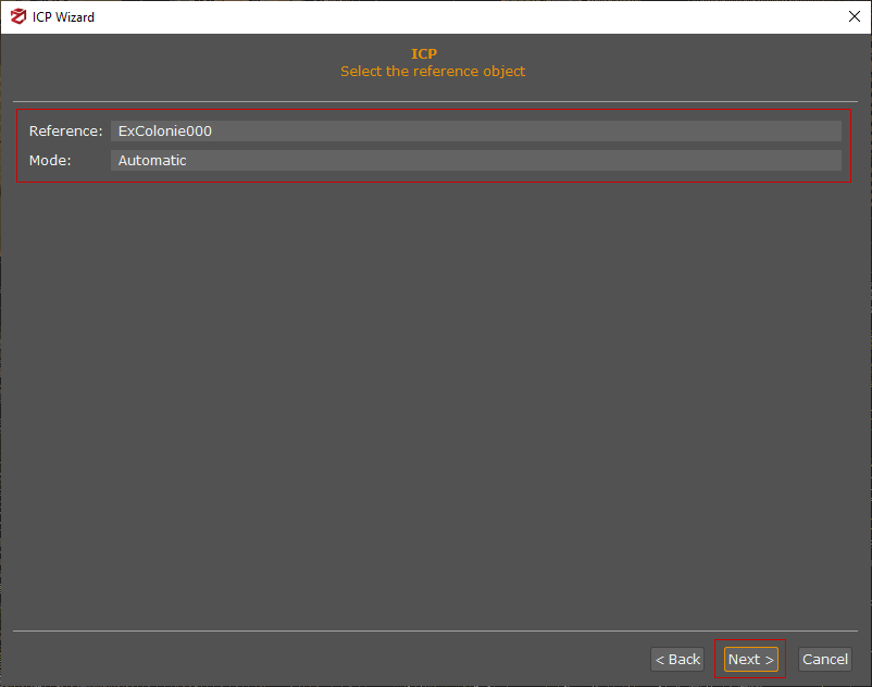
In the Select the reference object page, you can select which scan will be used as a Reference and the Mode based on how the scans have been captured; the default option is set to “Automatic” . Click the “Next” button to continue.
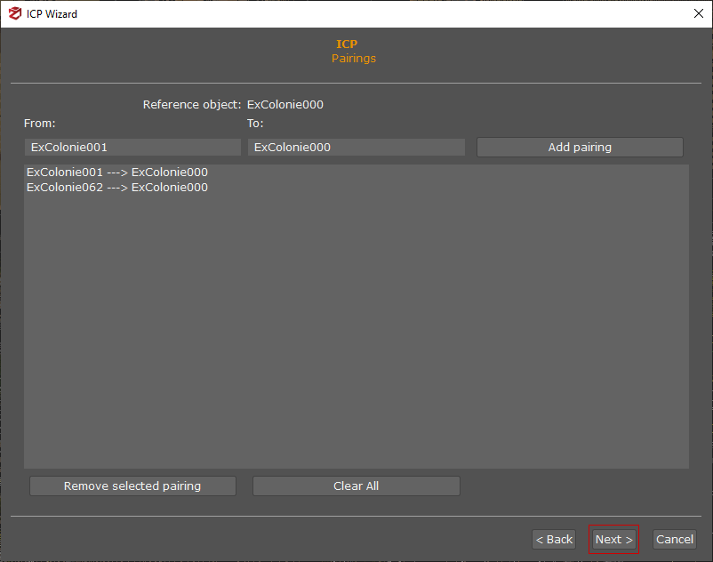
On the Pairings page, you can define the object pairings. In most cases, the pairings should not be changed, as they should be selected automatically, and no further user interaction is required. Click the “Next” button to continue.
On the Parameters page, you can tune the ICP algorithm settings according to the initial, rough alignment and the properties of the laser scans (e.g., the amount of noise coming with the scans).
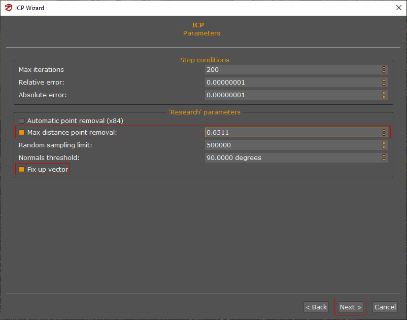
Parameters are explained in detail below:
-
– Max Iterations: This is the maximum number of iterations on the base to which the ICP will be applied.
– Relative error: Difference between the error of the current iteration and the error of the previous iteration.
– Absolute error: current iteration error
The two parameters above can be modified to set an acceptable error threshold where iterations can end before reaching the maximum number (max iterations). This saves processing time, especially in the case of very large numbers of scans that are already fairly aligned.
– Automatic point removal (x84): Distance automatically calculated to discard outliers
– Max distance point removal: This distance is expressed in the unit in which the original scans were taken. The reference scan as the origin, can be used to exclude all points further away than a certain number of units.
– Random sampling limit: Sample of points used by the algorithm to perform the ICP. In the case of large scans, this parameter can be used for considering only a sample of points from the total to perform the alignment.
– Normal threshold: Maximum difference between accepted point normals. It can be used to improve point correspondences in certain borderline cases
– Fix up vector: Fixes the z-axis and allows rotation only on that axis. The vertical Z axis of a scan is usually always correct, so enabling the checkbox allows to have one less variable to calculate during the ICP.
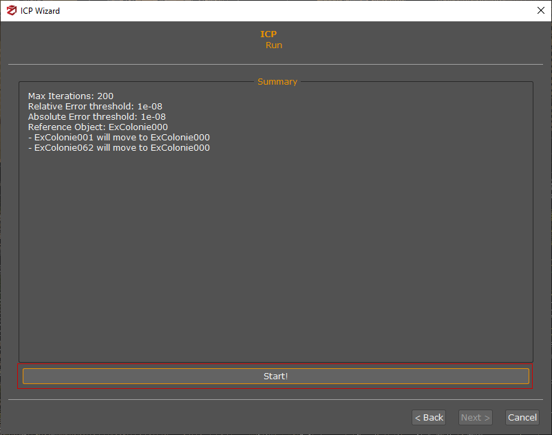
Click the “Next” button and the Run page will recap the overview information. You can start the actual computation by pressing the “Start!” button.
When the computation has finished, a Global residual histogram will be shown on the screen:
-
– Points represent the number of points on the Y-axis;
– Residuals represent the residual error on the X-axis.
The histogram is calculated based on Euclidean point-plane distance, which tends to lead to lower error values; in relation to the point-point distance. The histogram is a global indication of the error trend in the registration of the scans. In case the scans are still very far from each other, the histogram will have high errors for many points. The raw alignment and the Multi-ICP with different thresholds can be repeated to lower the error,.
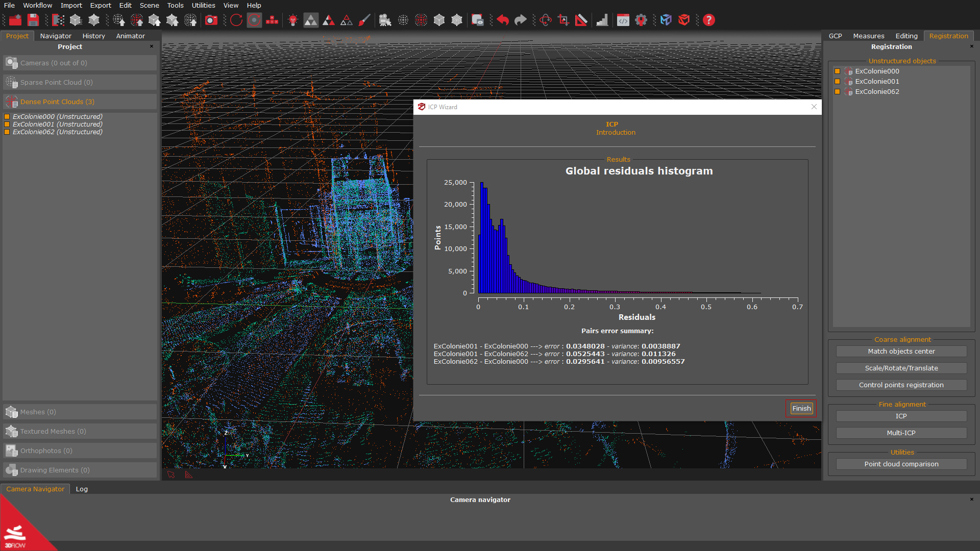
You will complete the Fine registration step by clicking on the “Finish” button.
Step 3 – Laser scan merging (optional)
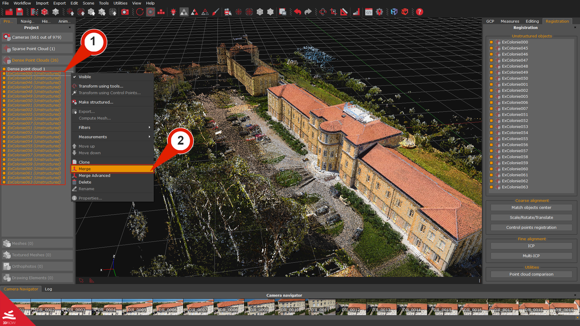
To better manage the next steps, merging all the registered scans is recommended before moving on. Select all the unstructured scans in the Project panel (1), right-click them, and pick the “Merge”(2) option.
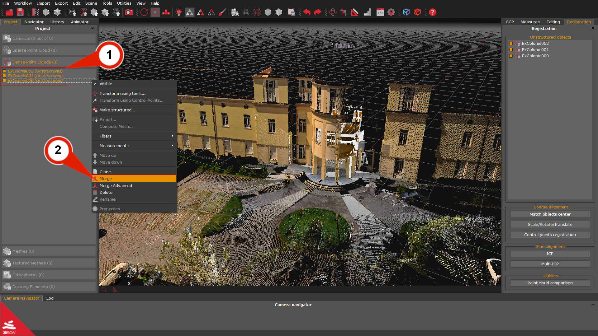
Congratulations! You have registered and merged all your scans.
Step 4 – Making laser scans structured
When you import LiDAR scans into 3DF Zephyr, they will result in unstructured point clouds.
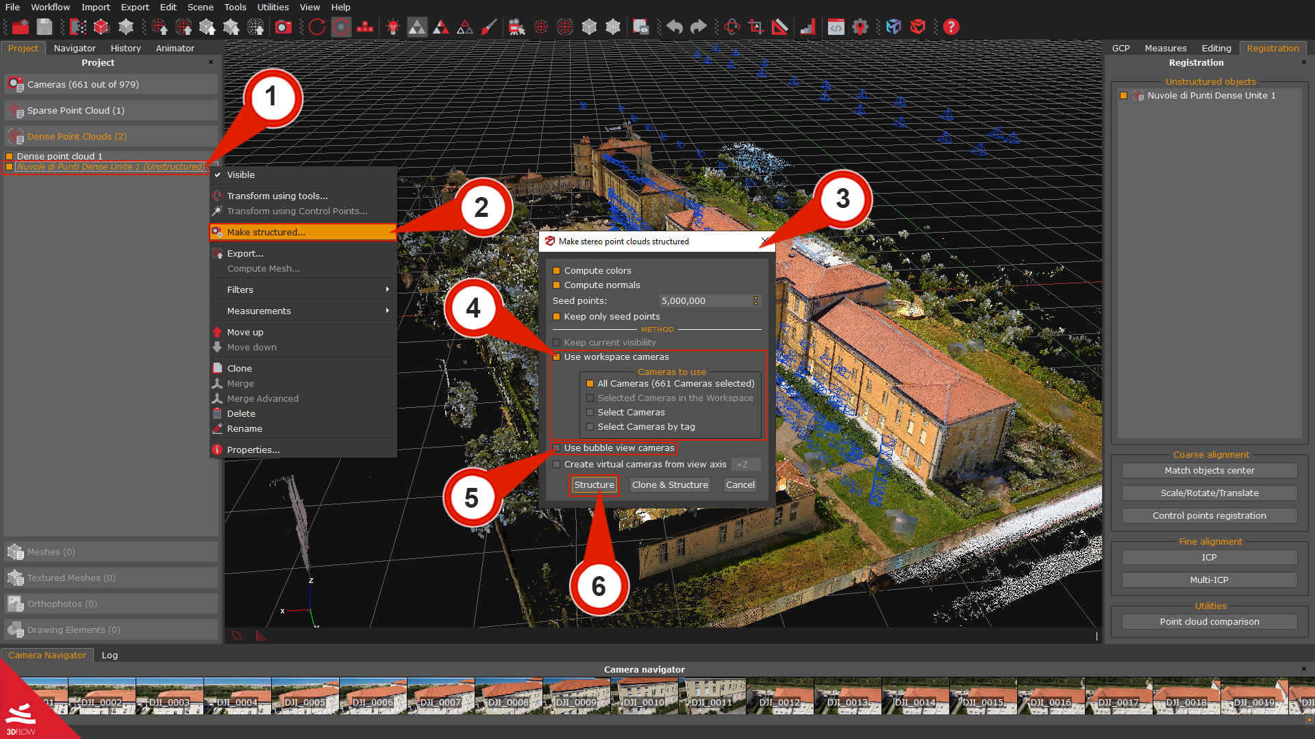
To start the workflow, right-click the unstructured scans (1) in the Project panel and select the Make structured (2) option; the “Make stereo point cloud structured” (3) dialog will appear.
> If you are dealing with data in native (.fls, .fws, .rdb, .rdbx, .zfs, .dp, .x3a) or .e57 format, be sure to enable the “Use bubble view cameras” (4) option and the appropriate settings (i.e., compute colors and normals).
> If you are dealing with data in a common file format (.ply, .pts, .ptx, .las, .xyz, .txt, .rcp, .laz), make sure that the “Create virtual camera from view axis” (5) checkbox is enabled.
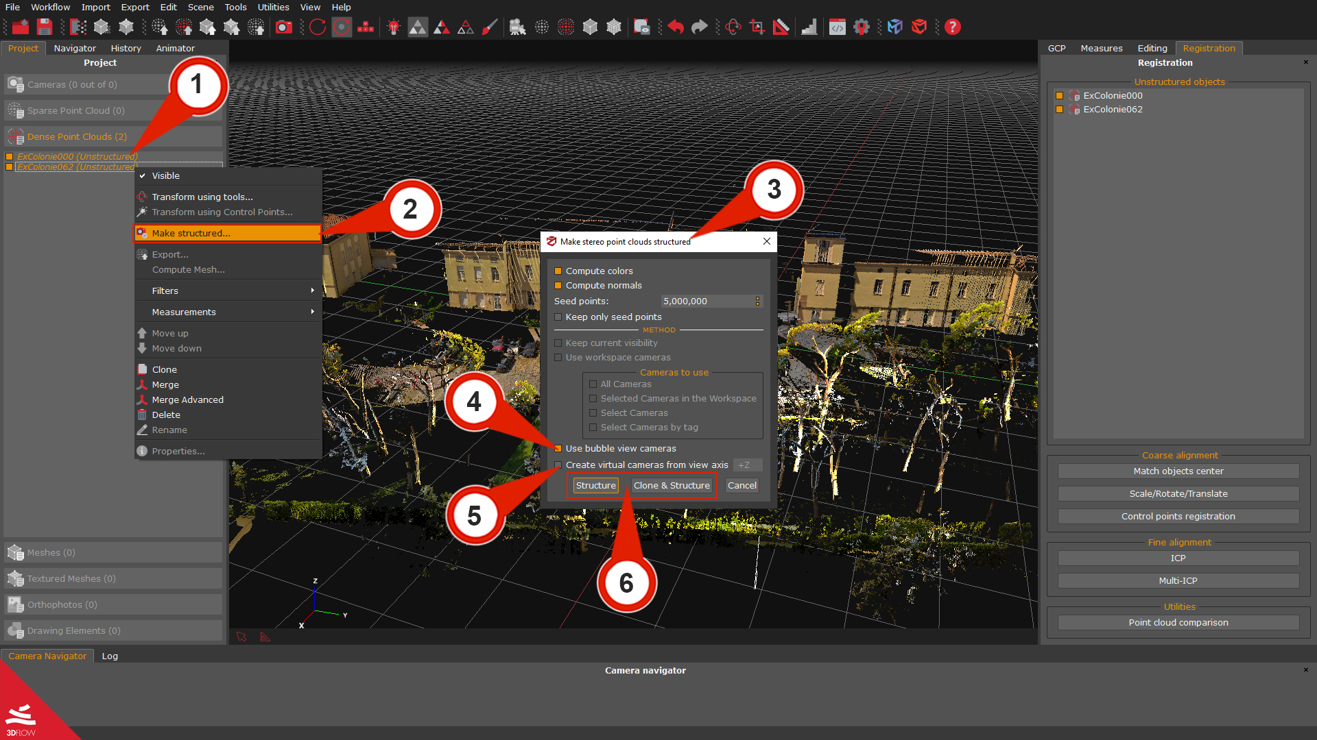
Note: It is possible to increase the number of the Seeds points, which are the points chosen by the mesh generation algorithm to retrieve more details on the mesh surface. They do not affect the structuring process directly.
Click the “Structure” or the “Clone & Structure” (6) buttons to start the process.
The new structured point cloud will be listed in the Dense point cloud section in the Project panel. It can be processed and manipulated just like a photogrammetry dense point cloud.
-
Section B: Automatic register images to scans
Laser scans need to be aligned before using this tool, so please refer to Section A: LiDAR data registration of this tutorial if they are yet to be registered.
Another requirement is that the scans must come with RGB data and origin coordinates (i.e., native file formats or .e57 format).
It’s possible to add UAV and/or ground pictures to a set of registered laser scans, which will remain fixed. The more laser scans, the more accurate the automatic registration tool.
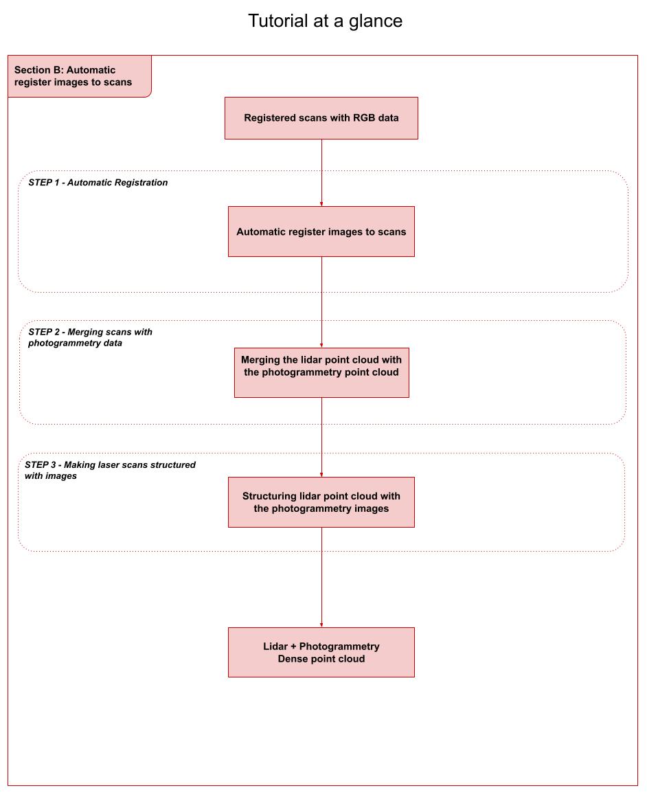
Step 1 – Automatic Registration
The tool is available from the Workflow menu > Advanced option >“Automatic register images to scans (1)”.
In the Input stereo point clouds (2) section, you can choose the registered laser scans to use as reference (it’s better to use many as possible).
The Input images (3) section allows searching the directory where the images are located, while in the Computation preset (4) section, you can set the reconstruction type category and preset according to the used case.
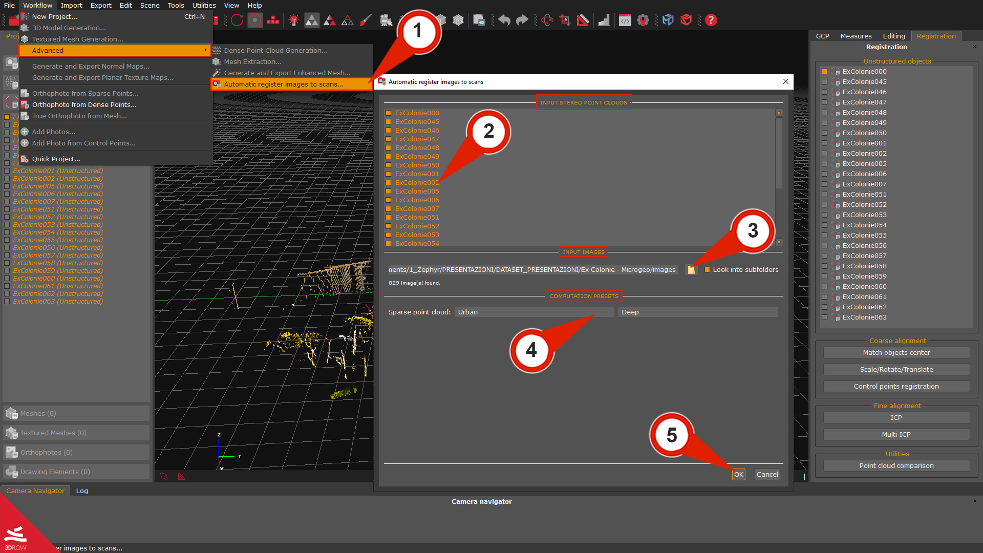
Once you are done with the settings, click the “OK” (5) button. A new sparse point cloud will be created and registered over the selected laser scans.
Note: in some cases, you can’t achieve a good result with the automatic registration; you can use sections Step 1 – Rough alignment
and Step 2 – Fine Registration to get your data registered.
In the video below you can watch a summary of the Automatic registration workflow:
Step 2 – Merging scans with photogrammetry data
Once done, you can create a dense point cloud starting from the photogrammetry sparse point cloud. Click the Workflow menu > Advanced > Dense point cloud generation to start the process.
Before or after the photogrammetry dense point cloud generation, you can select all the unstructured LiDAR scans (1) in the Project panel, right-click them, and pick the “Merge” (2) option.
The point cloud laser scan can now be either merged with the photogrammetric dense point cloud or kept separated, e.g., if you want to create a mesh and a textured mesh based on the LiDAR data.
Step 3 – Making laser scans structured with images
Unstructured point clouds are those whose origin is unknown by the software because they are imported as an external element into 3DF Zephyr.
When you are dealing with native laser scan format (.fls, .fws, .rdb, .rdbx, .zfs, .dp, .x3a) and e57, we can use the workspace cameras or the bubble view for generating structured point clouds where the aligned scans are “fixed” to the origin of the images data.
Select and right-click the unstructured scans (1) in the Project panel and then click the Make structured (2) option. The “Make stereo point cloud structured” (3) dialog will appear. The structuring process can be performed by linking scans to:
-
– photogrammetric images by enabling the “Use workspace camera” (4) checkbox.
– bubble view images by enabling the “Use bubble view camera” (5) checkbox;
Finally, you can set the appropriate options (i.e., compute colors and compute normals) and click on the “Structure” (6) button to start the process.
The structured laser scans can be processed and edited like any other point cloud element. You can merge them and the photogrammetry point clouds or directly generate a mesh from the LiDAR data.
-
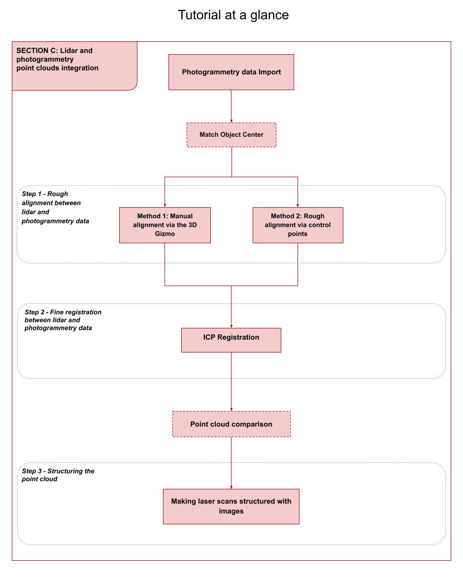
Section C: LiDAR and photogrammetry data integration
The last part of this tutorial provides guidelines for integrating LiDAR and photogrammetry data. It assumes that you have already registered the LiDAR scans using 3DF Zephyr or external software and have already generated a dense point cloud from images in your photogrammetry project. Also, laser scans and aerial/ground pictures are supposed to capture (more or less) the same scene or part of it in order to have some overlap for data registration.
Photogrammetry data Import
Return to summary
Open a new Zephyr session with the registered laser scans. Drag and drop the zep file, including your photogrammetry project, into the “laser scans” software session.
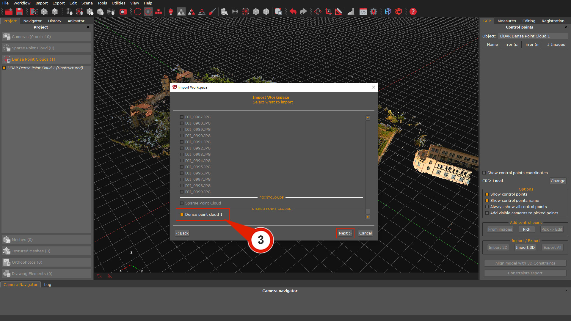
Click the “Merge” button in the pop-up window, and the Import workspace (1) window will appear. Make sure to select the “Same reference system (direct merge) (2)” option and click “Next”.
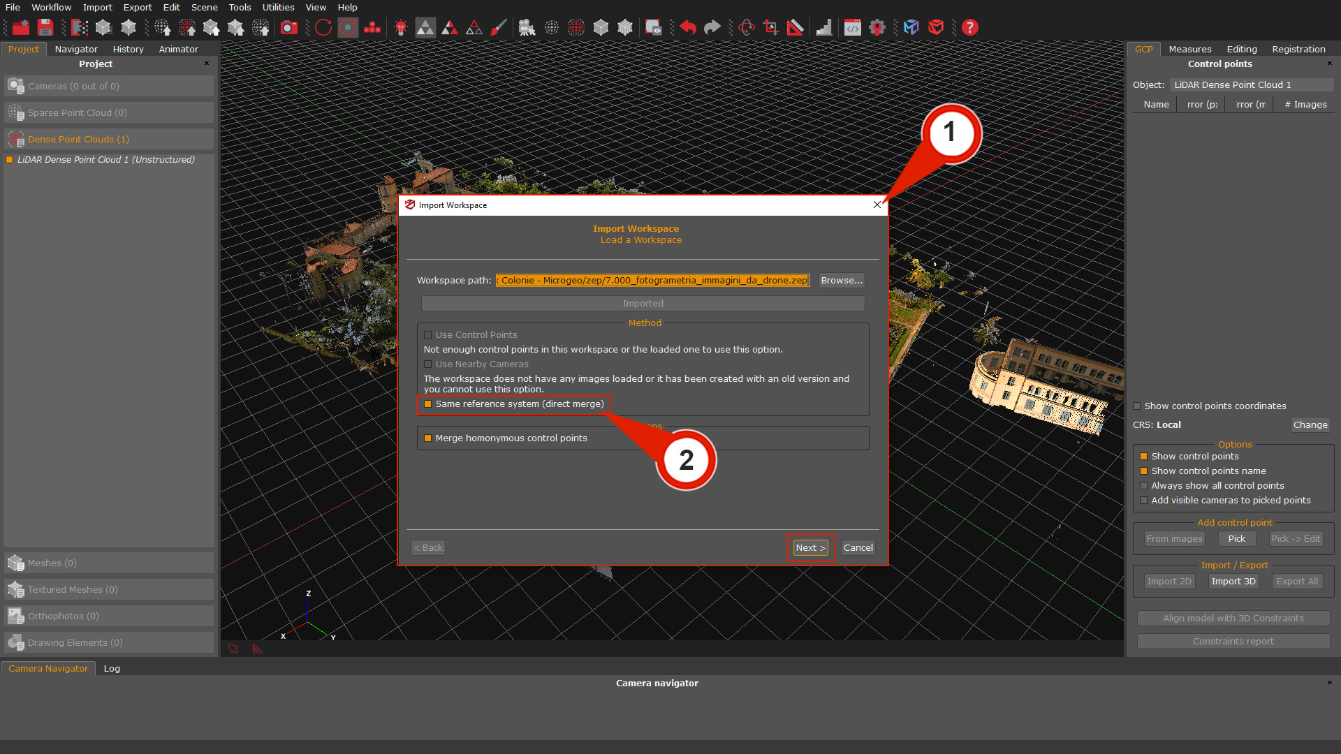
On the following page, you can choose the elements that will be merged in the project; in this case, the dense point cloud (3) check-box must be selected; click the “Next” button again. To complete the import process click the “Align” button.
The Match Object Center tool
Return to summary
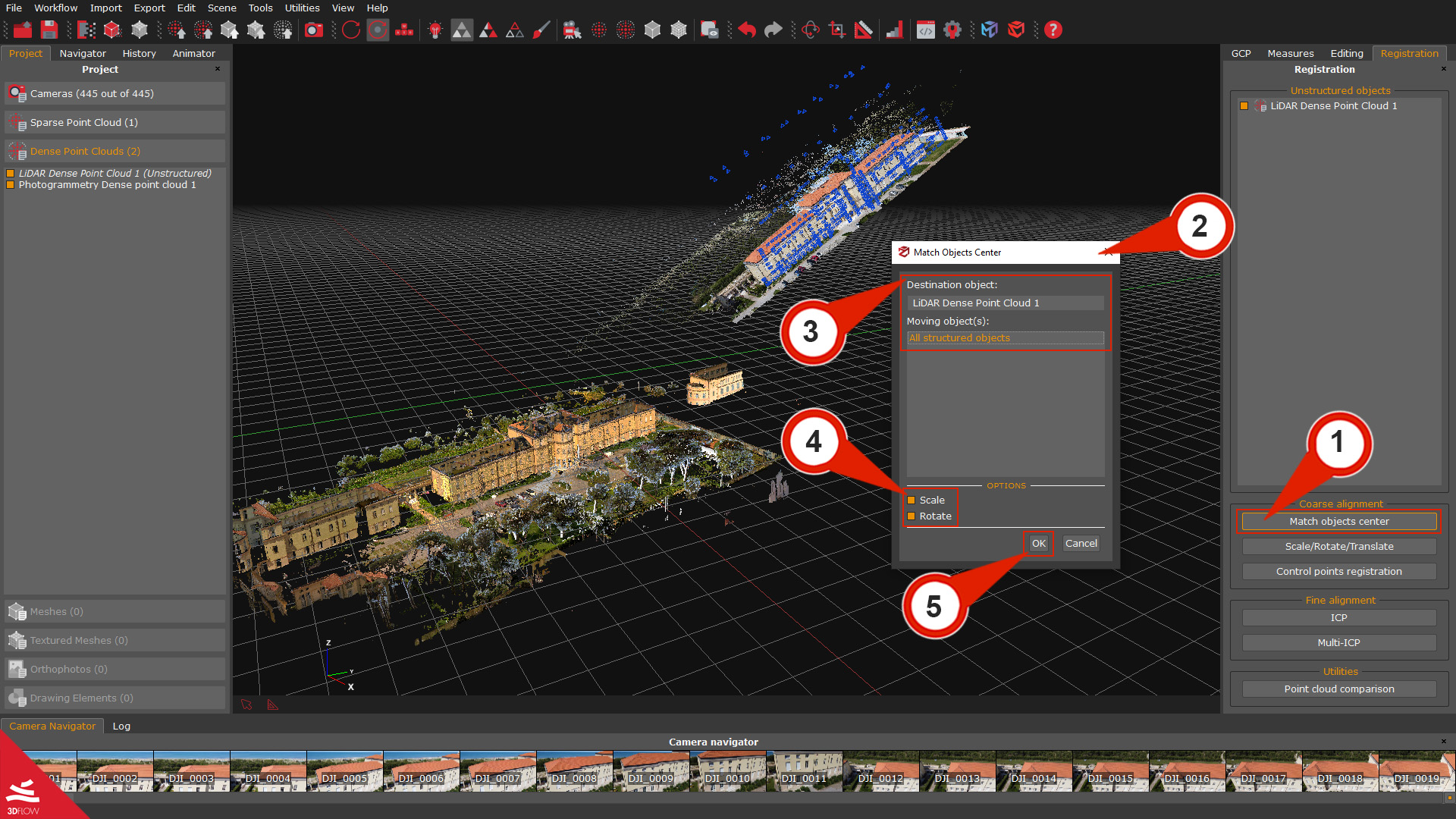
LiDAR and photogrammetry are often captured with different reference systems. This is why sometimes you don’t immediately see the photogrammetry point cloud you have just imported in the “laser scans” sessions. The “Match objects center” tool allows roughly translate and rotate the photogrammetry point cloud to the laser scans.
Click on the “Match Object Center” (1) button in the “Registration” panel on the right side of the user interface, the “Match Object Center” (2) window will appear. Select the “Destination object” (3) (typically, a laser scan) and the “Moving object” (3) (typically, the photogrammetry dense point cloud).
Make sure to enable the Scale (4) and Rotate (4) checkboxes to get the best match between the subjects. Click the “Ok” (5) button to apply the transformation.
Step 1 – Rough alignment between LiDAR and photogrammetry data
Method 1: Manual alignment via the 3D Gizmo
You can use the Gizmo to bring the scans and the photogrammetry point cloud to a rough alignment. You can enable the “Gizmo tool” from:
– The Registration tab is on the user interface’s right side; by clicking the “Scale/rotate/translate (1a)” button.
– By clicking the “Scale/rotate/translate objects (1b)” button in the top toolbar.
– By right-clicking the target photogrammetry point cloud and choosing the “Transform using tools (1c)” option.
The “Transform object” (2) window will appear.
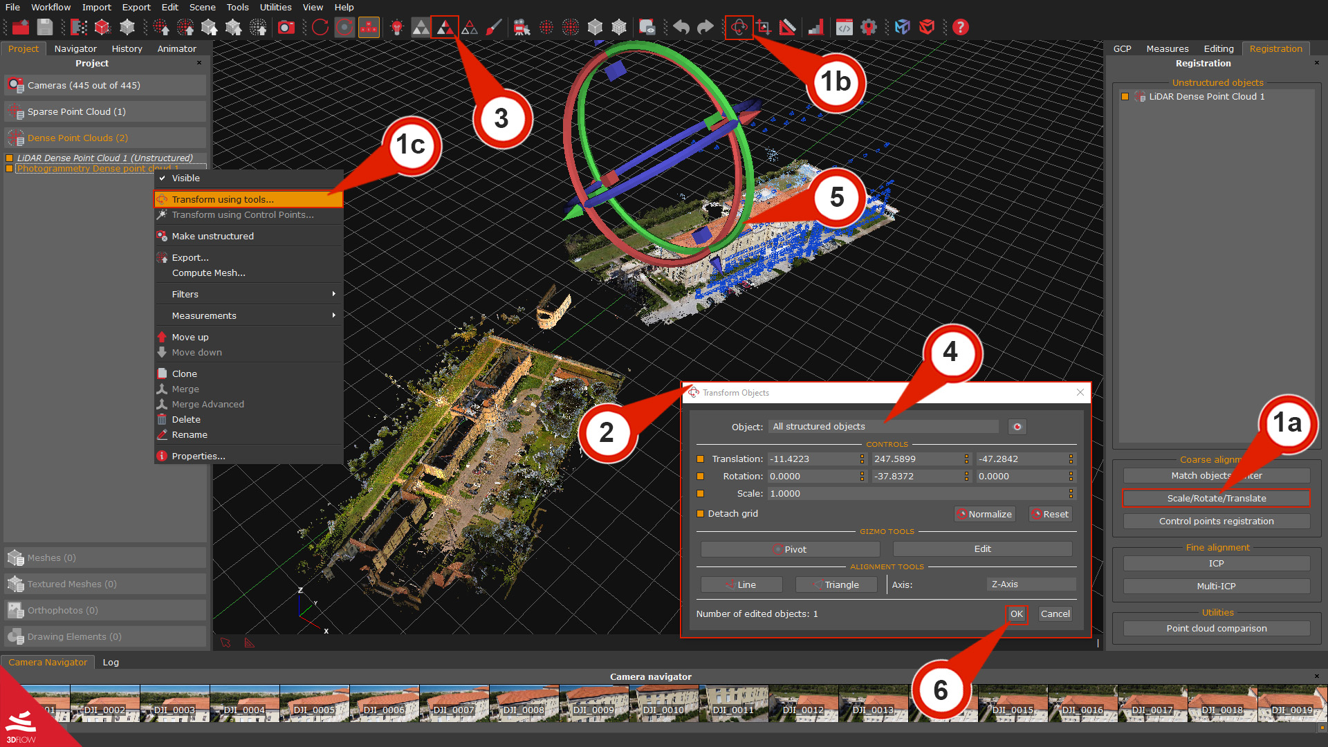
When using the 3D gizmo, please notice that it’s better to enable the visualization of all the desired items using their related checkbox in the Project tab before starting the rough alignment. To ease the alignment visualization, you can also enable the “Uniform colors” (3) view by clicking the related button in the toolbar.
From the dropdown box “Object” (4), you can also select which point cloud will be moved using the Gizmo (5).
Once You have roughly aligned the photogrammetry point cloud to the LiDAR one, click the “OK” (6) button before exiting the gizmo tool to confirm the roto translation.
Method 2: Rough alignment via control points
The second method for aligning LiDAR point clouds with photogrammetry data involves using control points. This approach considers translation, rotation, and scale to ensure accurate alignment.
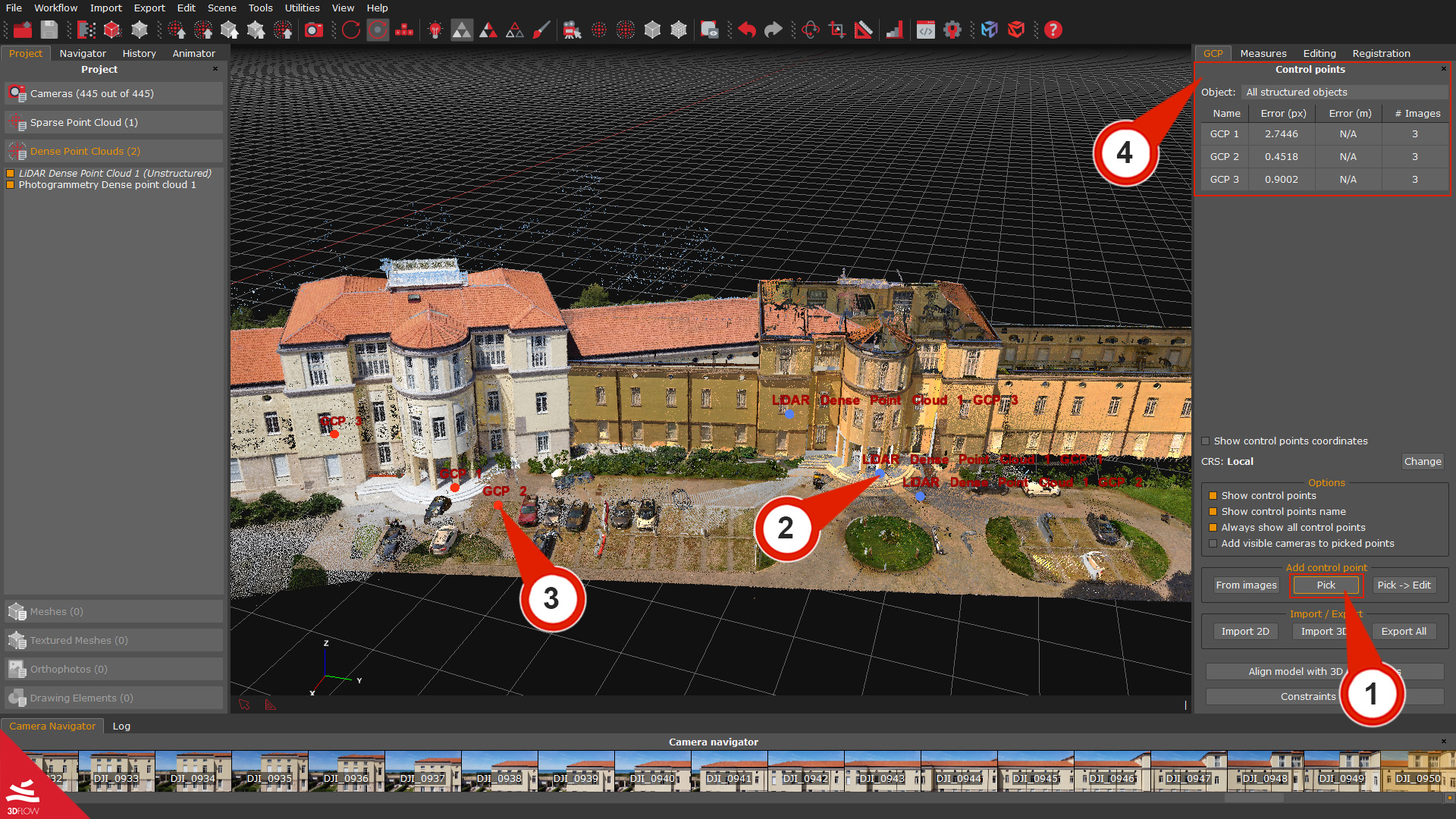
Click the “Pick” (1) button in the GCP panel and place at least three control points (2) on the LiDAR point cloud. Then, use the “Add control point from images” tool to locate and set the corresponding control points over the photogrammetry point cloud (3).
Note: Please, make sure to place the control points on the same areas that you can recognize easily on both laser scans. Usually, edges work very well. Keep in mind that it is better to select points that are located on all three axes.
The added control points will be listed in the GCP panel (4) depending on their reference object.
Once done, select the “Control point registration” (5) button in the Registration tab. The Control point registration wizard (6) will appear.
Click the “Next” button on the second page; you can select which object will be the Moving Object and which one will be the Fixed Object. Click on the “Next” button.
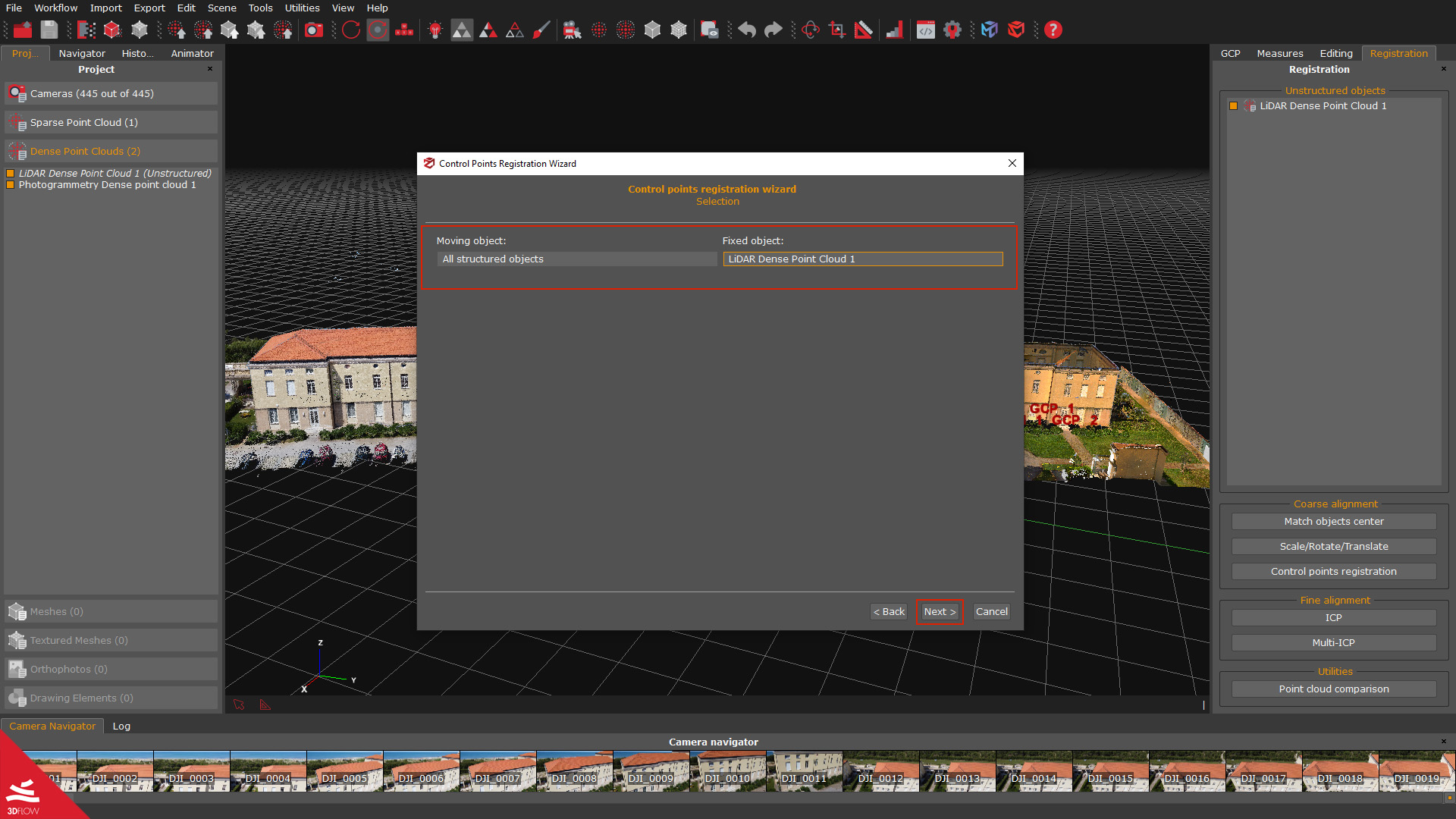
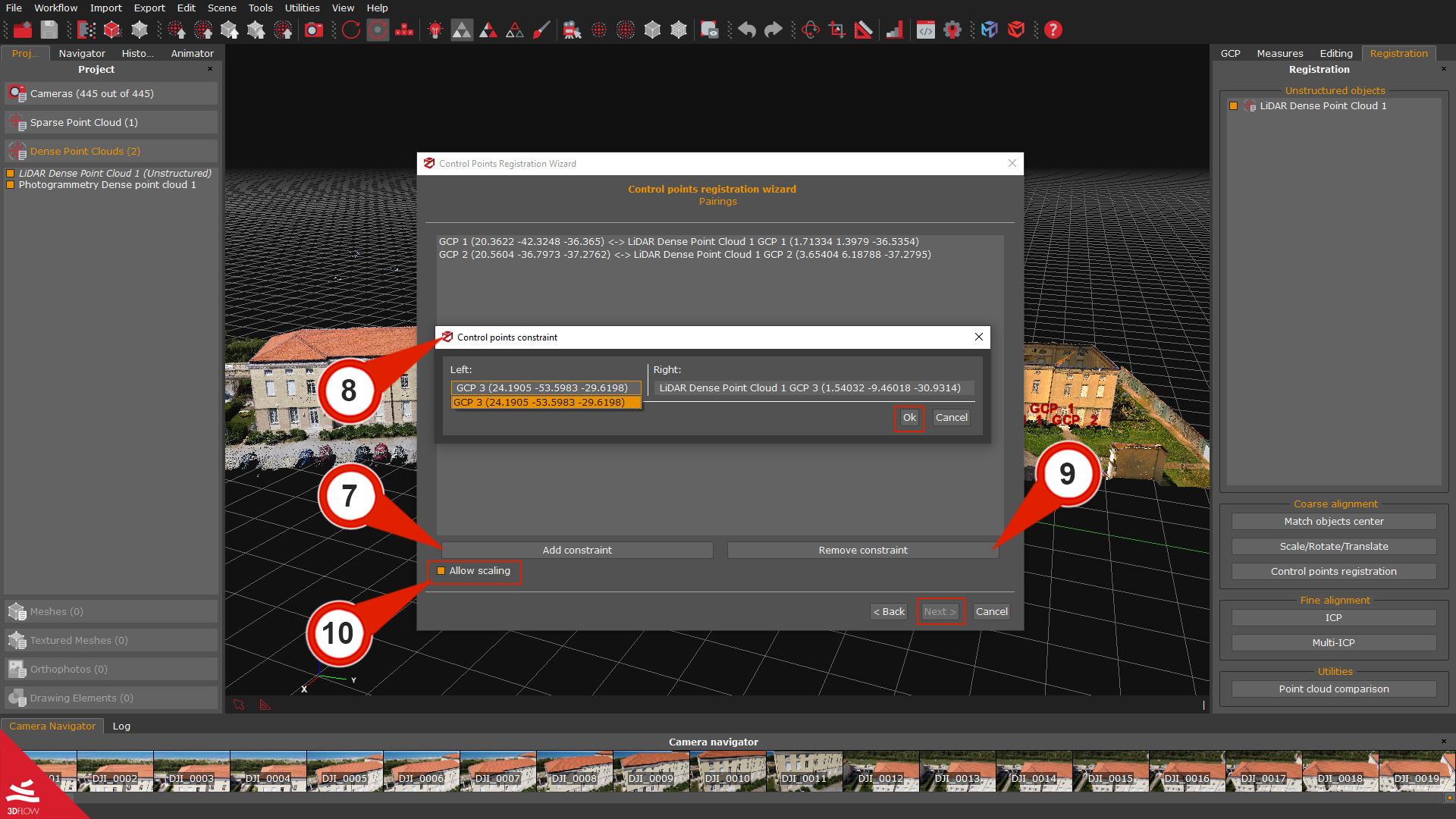
On the Parings page, use the “Add Constraint” (7) button to select the pairings (8) accordingly to the control points labels that you have previously used; at least three couples of control points are required.
It is also possible to remove the pairing using the “Remove constraint” (9) button, and before proceeding, it is also recommended to check the Allow scaling (10) checkbox.
Click the “Next” button and the “Apply” button on the next page to start the Rough alignment.
Step 2 – Fine registration between LiDAR and photogrammetry data
The ICP algorithm can be utilized to register the photogrammetry point cloud to the LiDAR point cloud, with the LiDAR point cloud serving as the reference.
-
> It is important to ensure that the objects are in close proximity to each other.
> The alignment and minimization process will be performed globally.
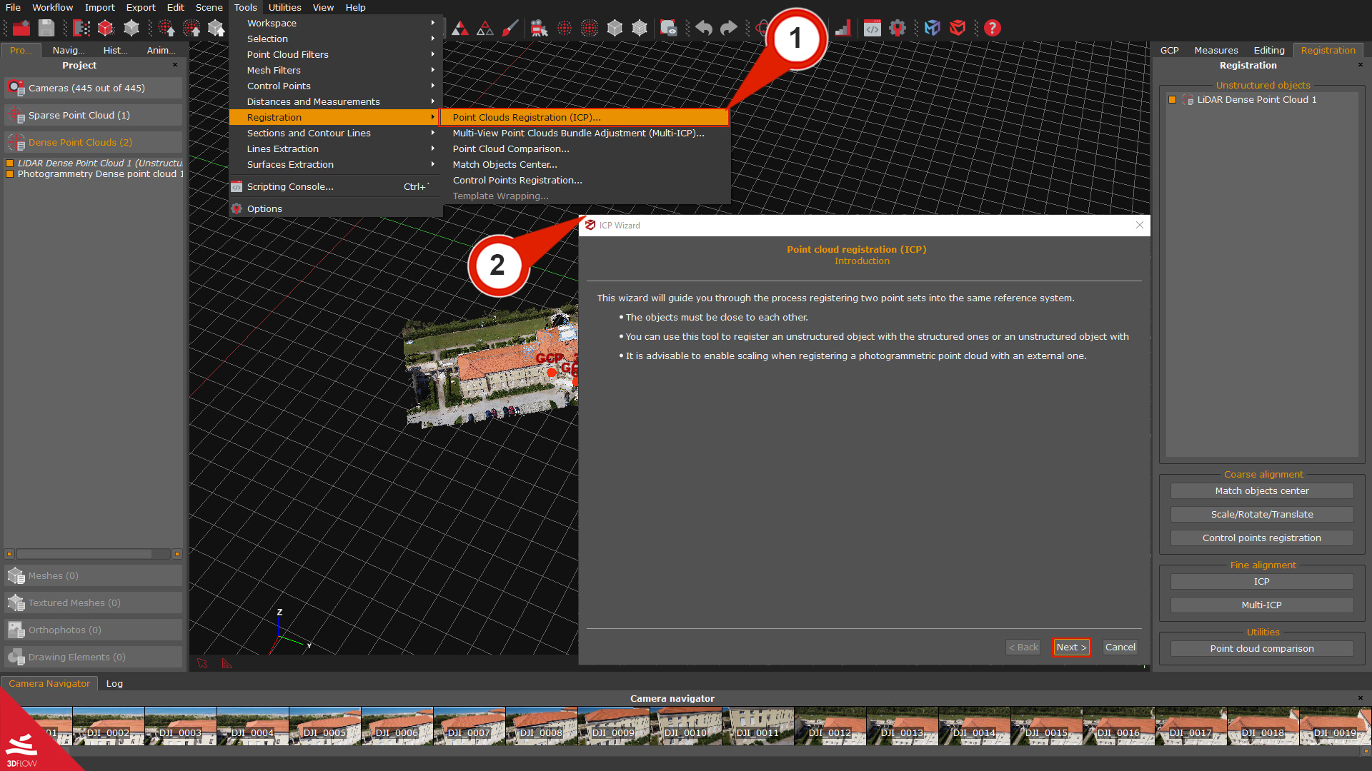
Click on Tools > Registration > Point Cloud Registration (ICP) (1) option, to open the ICP Wizard (2).
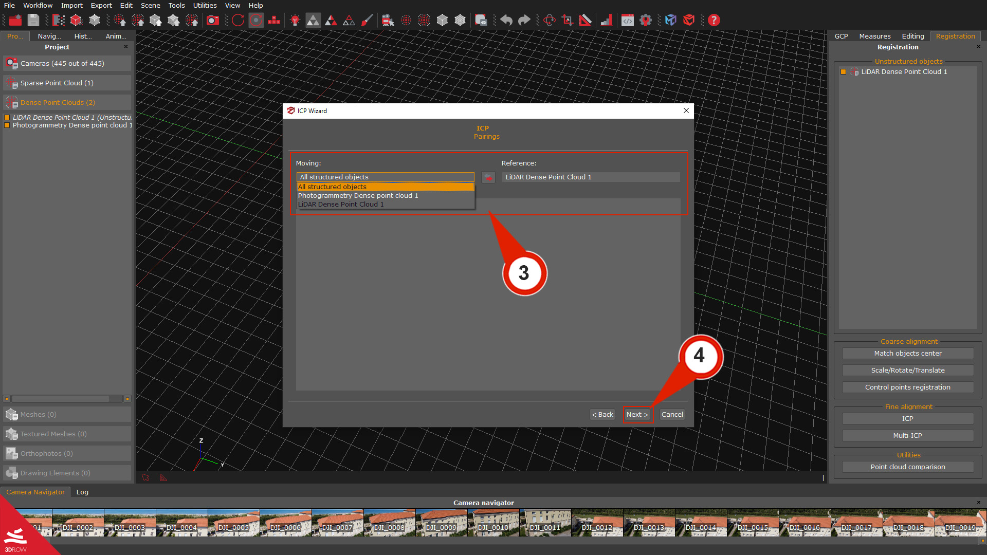
On the Pairings page, you can choose, as Moving objects, all the structured objects, and as Reference (3), the unstructured LiDAR point cloud. Click the “Next” (4) button to proceed.
On the Parameters page, you can set conditions according to which the algorithm will align the scans; if you encounter the need to align point sets with varying scales, it is advisable to activate the Enable scale adjustment check-box. Click the “Next” button to proceed.
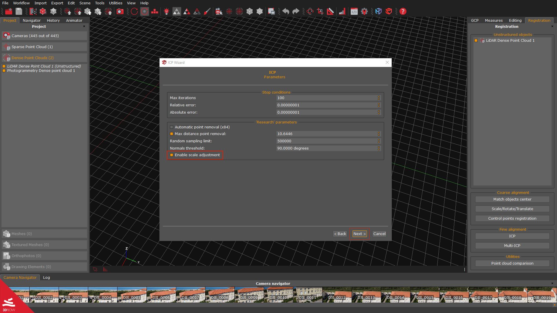
On the wizard Run page, click the “Next” button and a recap page will be shown where you can start the actual computation by pressing the “Start” button.
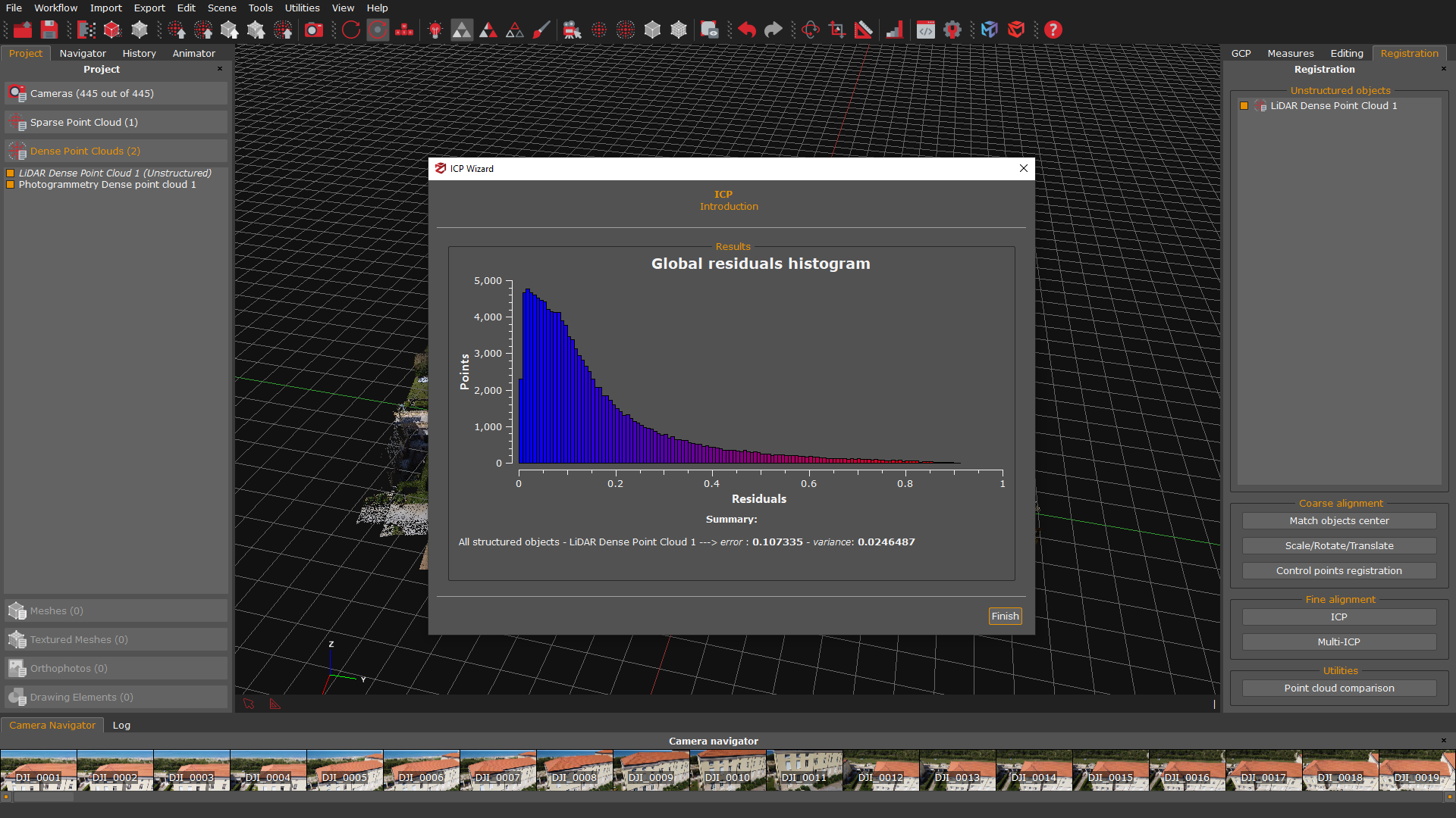
When the computation has finished, a Global residual histogram will be shown on the screen:
-
– Points represent the number of points on the Y-axis;
– Residuals represent the residual error on the X-axis.
The histogram is calculated based on Euclidean point-plane distance, which tends to lead to lower error values; in relation to the point-point distance, and represents a global indication of the error trend in the registration of the point clouds. In case the scans are still very far from each other, the histogram will have high errors for many points. The raw alignment with GCPs and another ICP registration with different thresholds can be repeated to lower the error.
Point cloud comparison (optional)
Once you are done with data registration, you can check the accuracy level of the registration and its error trend by leveraging the Point cloud comparison tool. The comparison is based on the distance between the vertices of the compared point/mesh clouds; by default, it uses the Euclidean point-to-point distance.
Cloud comparison parameter settings are as follows:
– Distance type: indicates the distance to be calculated, and users can choose either “point to point” or “plane to point” distance;
– Farthest points removal Distance: represents the highest value during the histogram computation;
– Number of Bins: defines the histogram amount of columns;
As for the residuals computation process:
-
– The first step computes the closest point of the model for every point of the target;
– If a distance between a couple of points is greater than the maximum distance value, that distance won’t be considered in the computation;
It is also possible to select parts of the histogram to highlight only a certain number of points of the “model” point cloud directly in the 3D workspace.
In the Point to point comparison, the histogram is built by considering the closest point A for each point B. All the spatial distances from A to B are used to build the histogram and color the point cloud accordingly. The Plane to point metric is a bit different. In this case, a plane is fitted considering B and its neighbors. The distance is then calculated from A to the fitted plane.
To start the comparison, click on the “Point Cloud Comparison” (1) button in the Registration tab on the right to open the Point Cloud Comparison (2) window.
Select the Reference (e.g., A laser scan) and the Model (e.g., the photogrammetry point cloud) (3). Set the Farthest points removal distance (4) and click the “Compute residuals” (5) button.
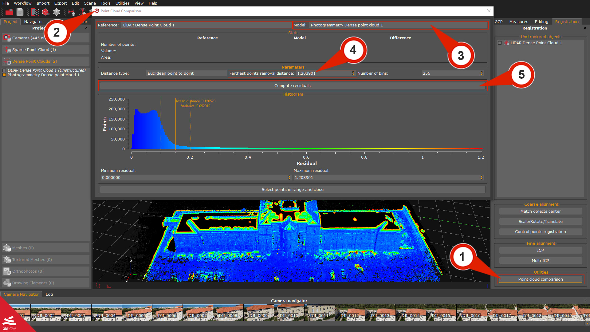
The tool will display a histogram at the end of the process::
-
> X-axis = Number of points
> Y-axis = Distance between points (residual).
You can check the error values at the bottom of the window (mean distance and standard deviation).
The color of the “model” point cloud will be updated in the 3D workspace according to the color pattern of the histogram, which will be very useful in pinpointing the most and less accurate – in terms of registration – areas of the point cloud you have considered.
Step 3 – Making laser scans structured with images
This last step allows structuring the point clouds with photogrammetry images.
The structuring process enables the generation of a structured point cloud in which aligned scans are “fixed” to the data origin. As for terrestrial lidar scans, this corresponds to the center of the laser scanner (bubble view); therefore, the structuring process allows Zephyr to link images to the scan and treat laser scans as photogrammetric point clouds.
To start the workflow, right-click the unstructured scans (1) in the Project panel and select the Make structured (2) option; the “Make stereo point cloud structured” (3) dialog will appear.
-
> If you are dealing with data in native (.fls, .fws, .rdb, .rdbx, .zfs, .dp, .x3a) or .e57 format, be sure to enable the “Use workspace camera” (4) or the “Use bubble view cameras” (5) option and the appropriate settings (i.e., compute colors and normals).
> If you are dealing with data in a common file format (.ply, .pts, .ptx, .las, .xyz, .txt, .rcp, .laz), make sure that the “Use workspace cameras” (4) checkbox is enabled.
Click the “Structure” or the “Clone & Structure” (6) buttons to start the process.
Note: It is possible to increase the number of the Seeds points, which are the points chosen by the mesh generation algorithm to retrieve more details on the mesh surface. They do not affect the structuring process directly.
The new structured point cloud will be listed in the Dense point cloud section in the Project panel. It can be processed and manipulated just like a photogrammetry dense point cloud.