Tutorial #A01 : Manage control points and distances in 3DF Zephyr
Using control points and distances
Welcome to the 3DF Zephyr tutorial series.
This tutorial will teach you how to use Ground control points (GCP), constraints, and control distances with 3DF Zephyr.
This tutorial cannot be completed with 3DF Zephyr Free or Lite versions.
Summary
Introduction
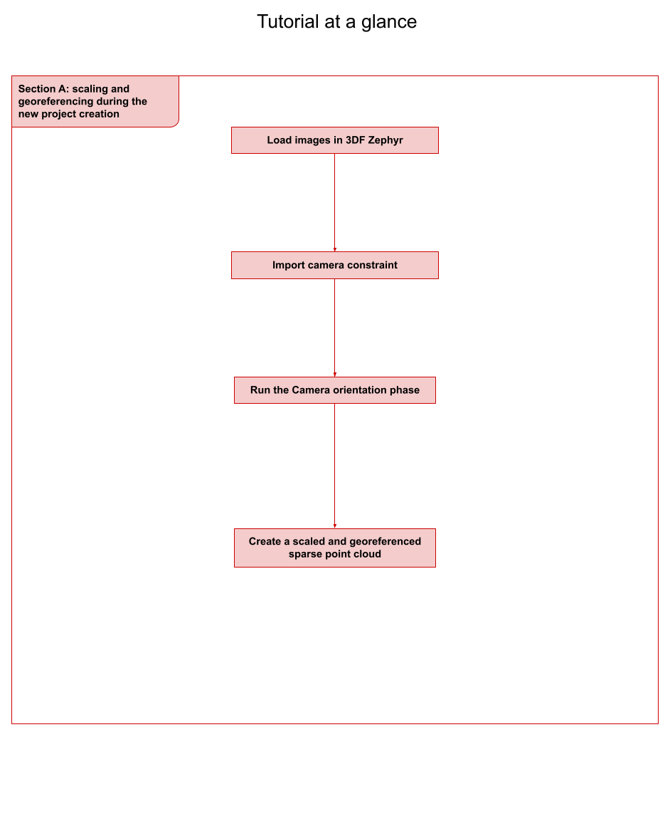
Section A: scaling and georeferencing during the new project creation
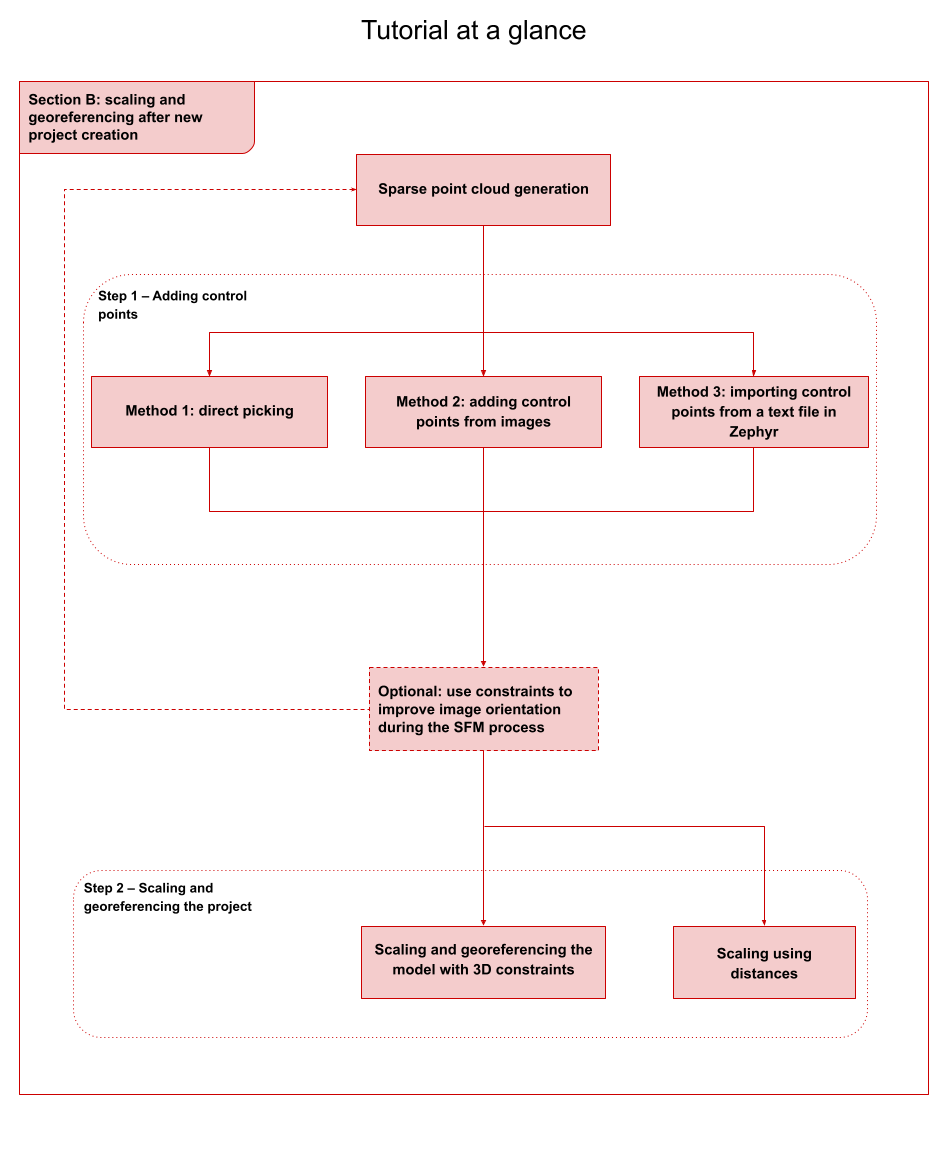
Section B: scaling and georeferencing after new project creation
Optional: use constraints to improve image orientation during the SFM process
Step 2 – Scaling and georeferencing the project
– Step 1 – Adding control points
– Optional: use constraints to improve image orientation during the SFM process
– Step 2 – Scaling and georeferencing the project
This tutorial is organized into two sections:
Section A: scaling and georeferencing during the new project creation
This workflow will explain how to use camera position coordinates during the new project creation workflow. In fact, 3DF Zephyr automatically detects pictures taken by UAV, leveraging their GPS or RTK coordinates to scale and georeference-created point clouds and meshes.
Note: It is always worth using at least one Ground Control Point (GCP), even when dealing with RTK imagery, in order to be aware of the ground accuracy.
Section B: scaling and georeferencing after new project creation
After creating a new project, it’s possible to use Ground Control Points (GCPs) for scaling and georeferencing the project in Zephyr by linking them to distances and GNSS coordinates collected on-site. GCPs can also be used to optimize the camera positions by leveraging the Bundle Adjustment algorithm, thereby reducing the reprojection error of images. Ground Control points, alignment, and model scaling with known control points (or known distances) can be managed from the panel on the right labeled GCP.
Remember that any reconstruction is up to an arbitrary scale factor, a translation, and a rotation!
To complete this tutorial, you can either use your dataset or download the sample .zep project you will find below.
 | Download Tutorial Dataset – 3DF_Zephyr_A01_Control_Points (1 GB) |
Importing image coordinates during the project creation
To set constraints by importing geographic positions from images as part of the workflow for creating a new project, you should activate the “Control points camera constraints” check-box on the first page of the New Project Wizard.
Note: If your images include RTK coordinates, 3DF Zephyr will automatically find them in the picture’s Exif data, setting the camera position accuracy accordingly.
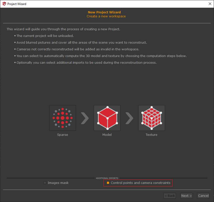
The Import Constraint page will follow the Camera calibration page.
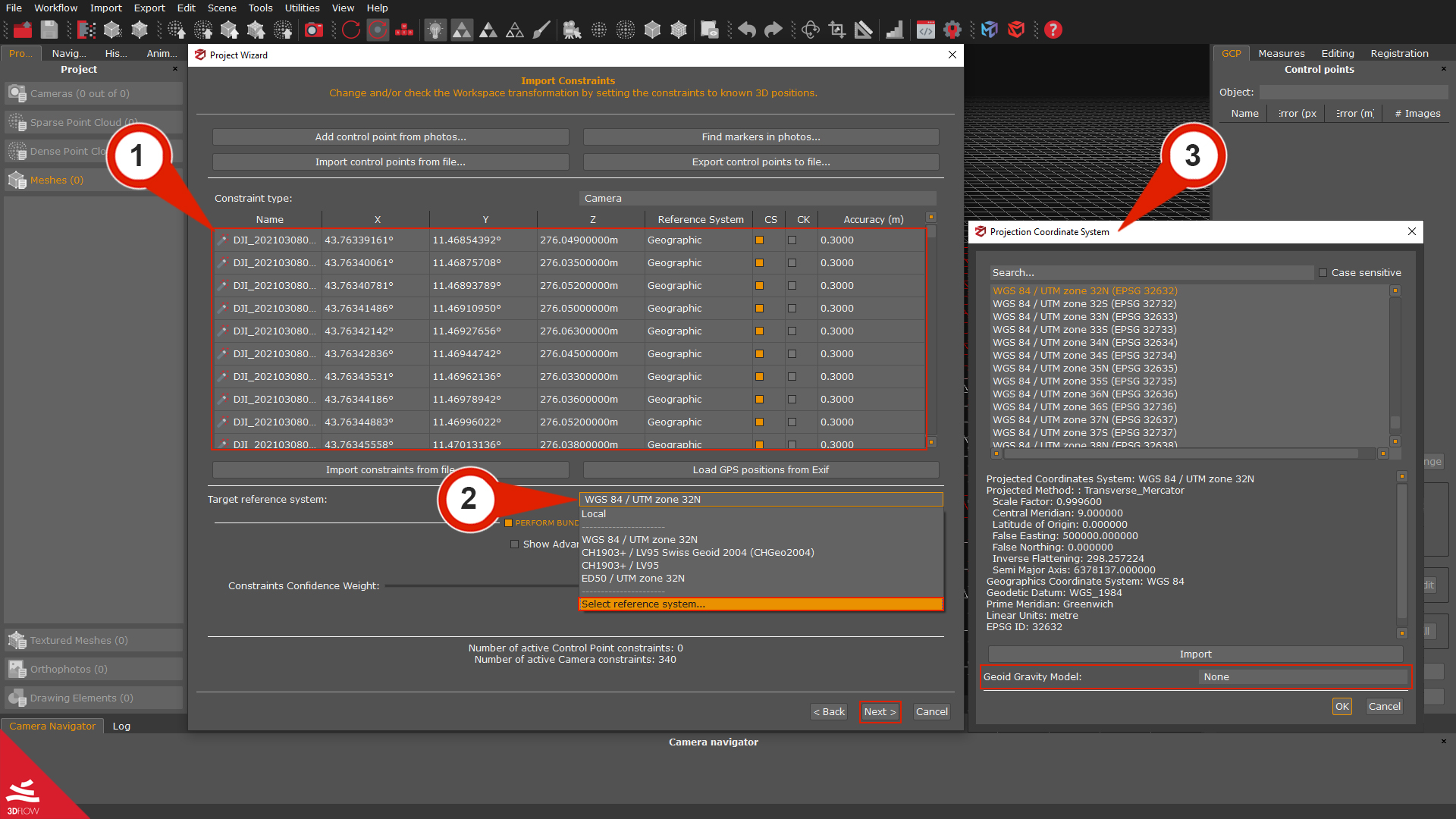
In the center section of the window, you can find a display of all the images loaded in Zephyr (1), along with their corresponding geographic coordinates. Unless there are specific requirements, it is generally sufficient to keep the default settings.
In other cases, you can press “CTRL+A” to select all the rows and right-click them. This action will open a context menu where you can choose from various options, such as:
– Setting the selected images as Constraints (CS) or Checkpoints (CK).
– Changing the Reference system, which refers to the coordinate system used for the project.
– Adjusting the Accuracy of each camera.
The software will also select the Target reference system (2) corresponding to the input coordinates. However, you can click on the Reference System drop-down menu and select the desired coordinate system from the “Select reference system” option to open the Projection Coordinates System (3) window. It’s possible to select the new coordinate reference system from the 3DF Zephyr database or import a new one from an external source by clicking the “Import” button and clicking “OK”.
A Geoid Gravity Model can also be downloaded and loaded in relation to the Coordinate Reference System. Following this link, you can download some of the most commonly used Geoids: https://www.3dflow.net/geoids/.
When everything is set, click the “Next” button to proceed to the following page of the project wizard. After the camera orientation process, the result will be a scaled and georeferenced sparse point cloud.
Step 1 – Adding control points
Method 1: direct picking
The easiest (yet the less accurate) way to add a control point is by picking it directly from the 3D reconstruction (on a point cloud or a mesh, but not on a textured mesh).
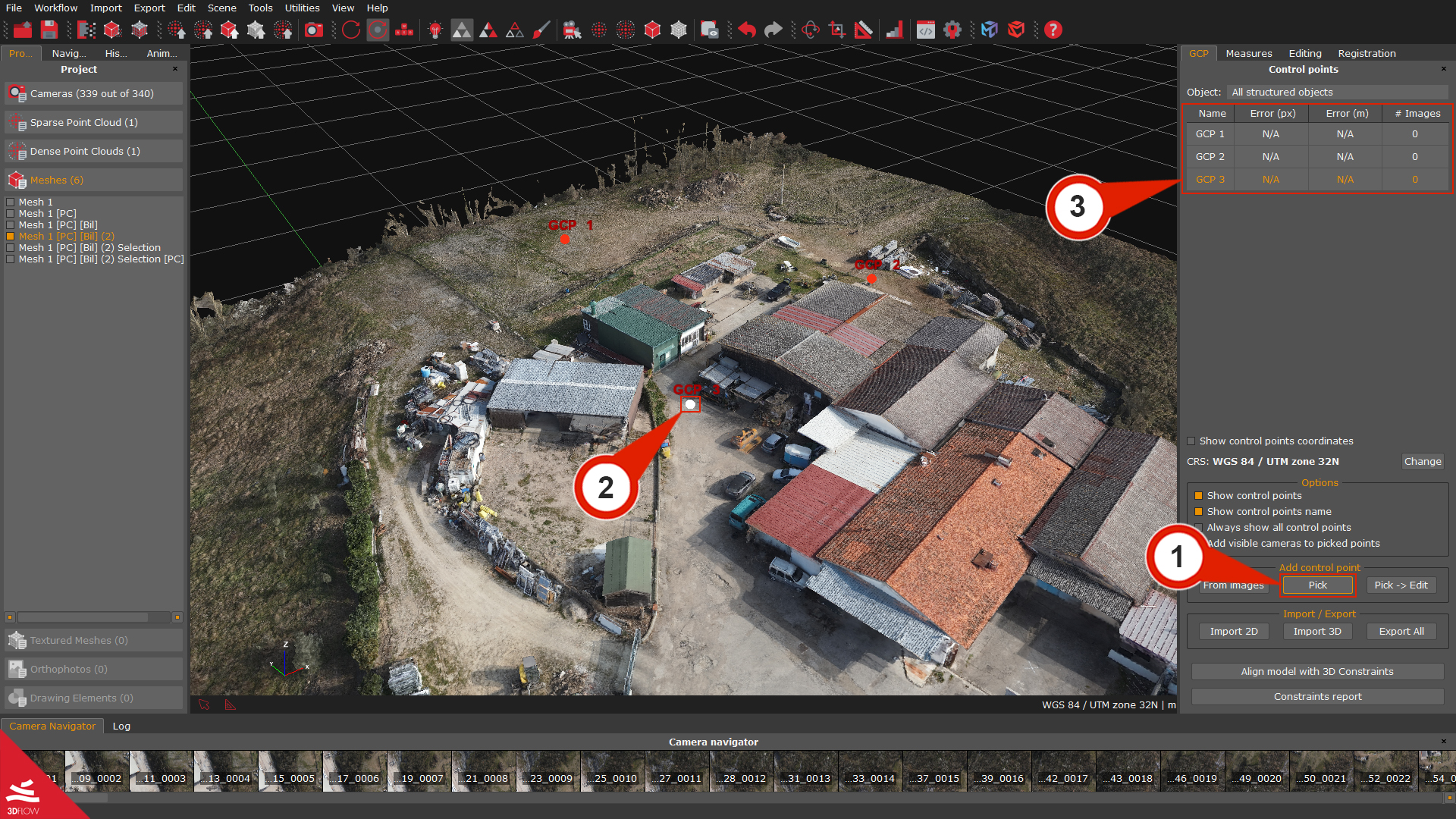
In the “GCP” Panel, click the “Pick Control Point” (1) Button. Your mouse cursor will turn into a crosshair icon: move the crosshair on the scene (2) and then left-click on the desired position. A new control point will appear in the Control Point List (3).
Of course, you cannot accurately place GCPs by direct picking on a sparse point cloud. You should use this method if you have created at least one dense point cloud.
Method 2: adding control points from images
A more accurate way to add control points is to pick them directly from the photos. You must place each control point on at least three pictures for the scaling process.
It is advisable to place it on as many pictures as possible if you plan to leverage control points to adjust the camera positions using the Bundle Adjustment optimization.
This method is suitable for dealing with a small/medium number of GCPs or images. For convenience’s sake, if you work with larger datasets (from about 2000 pictures upwards), you’d better rely on method #3 described below.
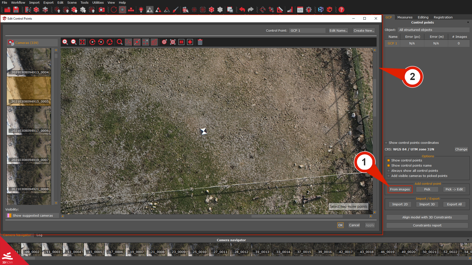
Click the “From images” (1) button from the GCP Panel to pick the Control Points. The “Control Point Editor” (2) will appear.
Please note that you can also click a camera in the 3D workspace (3) to select a camera in the camera navigator tab. Right-click on the thumbnail camera (4) to select the “add control points from images” (5) option and place the control point of the image you have chosen in the Control Point Editor (6).

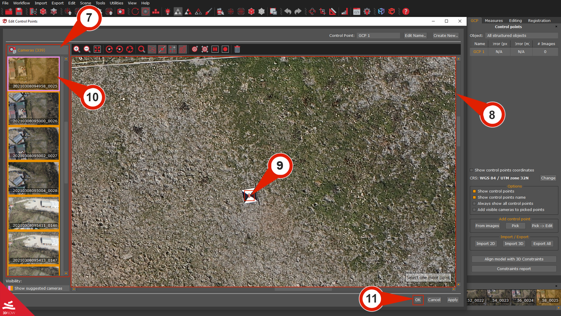
In the Camera list (7), left-click a picture to view it in the Control Point Picker Selector (8). Left-click where you want the control point, and a Red dot (9) will appear. A violet border will highlight the first selected image (10), but the “OK” (11) button won’t be available yet:
remember, at least two images to define a control point in the 3D space are needed.
Click again on another picture from the “Camera List” (7). You will notice an Epipolar line (12) before placing the control point, namely a further hint by Zephyr suggesting the control point you have previously placed is located somewhere in the picture along that line (13).
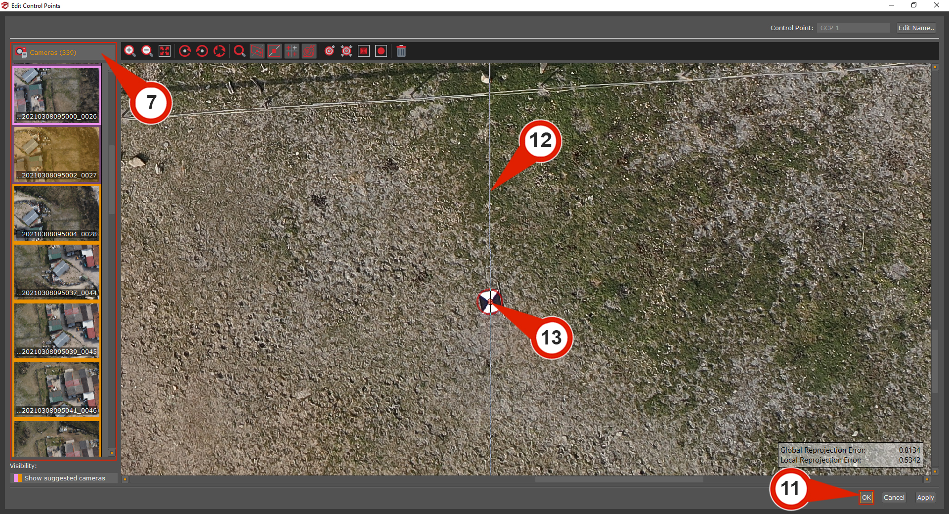
Remember to find the control points on as many pictures as possible if you plan to optimize the cameras’ orientation using the Bundle Adjustment. The more images involved, the more accurate the Bundle Adjustment will be. Click the “OK” (11) button to finish adding your new control point.
You can see the Global Reprojection error and the Local Reprojection error values (updated in real-time) while placing control points on the pictures.
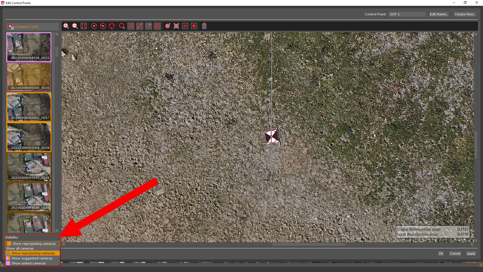
Camera Visibility
Once a control point has been placed on the first image, the Control point editor lists the most reliable cameras, according to Zephyr, by default. Sometimes slanting or too far cameras (from the picked point) are not included in the “Show suggested cameras” option selected, even though that point is visible on those cameras.
Depending on the onsite data capture (overlap between the pictures, nadiral, oblique capture, or both, etc.), it is advisable to select the “Show reprojected cameras” option to involve every pertinent image once you are done with the “Suggested cameras”. That will be crucial to run the Bundle Adjustment smoothly at a later time.
The Advanced Tools listed below will help you place control points on the pictures:
 | Fit in view: resize the image to fit in the view. |
 | Rotate 90 degrees clockwise, counter-clockwise, reset rotation: rotate the image and reset the initial position. |
 | Show magnifier: show/hide the magnifier on the cursor while placing control points on images. |
 | Show reprojection error: show/hide the current control point’s local and global reprojection errors. |
 | Show epipolar line: show/hide the epipolar line |
 | Show other points: show/hide previously placed control points. |
 | Automatic matching on current image: find and place a control point on the current image automatically. |
 | Automatic matching on all images: find and place a control point on all the pictures automatically. |
 | Detect marker: It automatically detects the center of a rectangular marker placed in the scene. By clicking the “Detect marker” icon and drawing a rectangle upon the center of the marker you want to be found, 3DF Zephyr will automatically place the control point at the center. Note: Using the tool with a check-board style marker will improve the automatic detection. |
 | Detect sphere: It allows the detection of the sphere’s center placed in the scene. By clicking on the “Detect sphere'” icon and drawing a rectangle over the sphere you want to be found in the image, 3DF Zephyr will automatically place the control point at the center. Note: This feature is expressly designed for the forensics industry, i.e., to support the analysis of the line of fire in crime scenes where a laser scanner scans the spheres on the trajectory rod. |
 | Clear point: remove control points placed on the image. |
Method 3: importing control points from a text file in Zephyr
Return to summary
If you are dealing with huge datasets and/or large numbers of control points, then importing GCPs at once rather than scrolling the whole set of images may be way more time-saving. Clearly, you still need to place control points on the images since what you have imported is not linked to the pictures yet. However, below, you will see the benefits coming with this method. To use this tool, please note that both the sparse point cloud you have created and the coordinates you want to import must have the same reference system. Coordinates from a .text or .csv file should be defined using the following syntax:
“Control_Point_1” 8.18880729e-01 -5.14516149e-01 4.54143586e-01
“Control_Point _2” -5.64690812e-01 -5.65085273e-01 1.09244112e+00
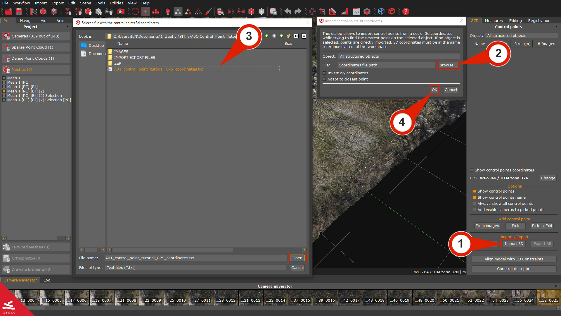
Click the “Import 3D” (1) button in the GCP panel to import 3D coordinates from an external file (.txt, .csv, .dxf).
Select the text file by clicking the “Browse” (2) button and make sure to pick the A01_control_point_tutorial_GPS_coordinates.txt (3) located in the sample dataset linked above. Click the “OK” (4) button to import the 3D coordinates.
The 3D coordinates will be added to the workspace as red points (5) and listed in the GCP panel:
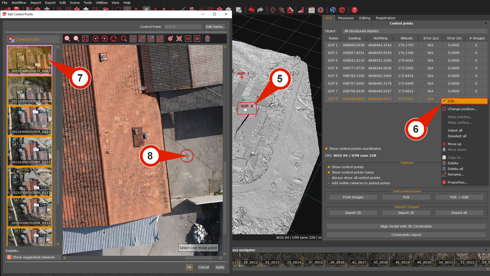
You have to link the imported control points to the pictures by right-clicking on each control point name in the GCP panel and selecting the “Edit” (6) option. In other words, by doing this, you are telling 3DF Zephyr the 2D coordinates of every control point. Once the Control point editor has opened, you will notice that 3DF Zephyr promptly suggests the cameras on which that point is visible in the Camera list (7). This means you can easily add the 2D point (8), avoiding browsing through the whole dataset.
This optional workflow is recommended for particular situations, where you can use the already-oriented cameras and their relative GCPs of a first Zephyr session, for enhancing the information available for the Structure from Motion (SFM) algorithm during the creation of a new project in a second session.
Consequently, this workflow will improve camera positioning and the resulting sparse point cloud.
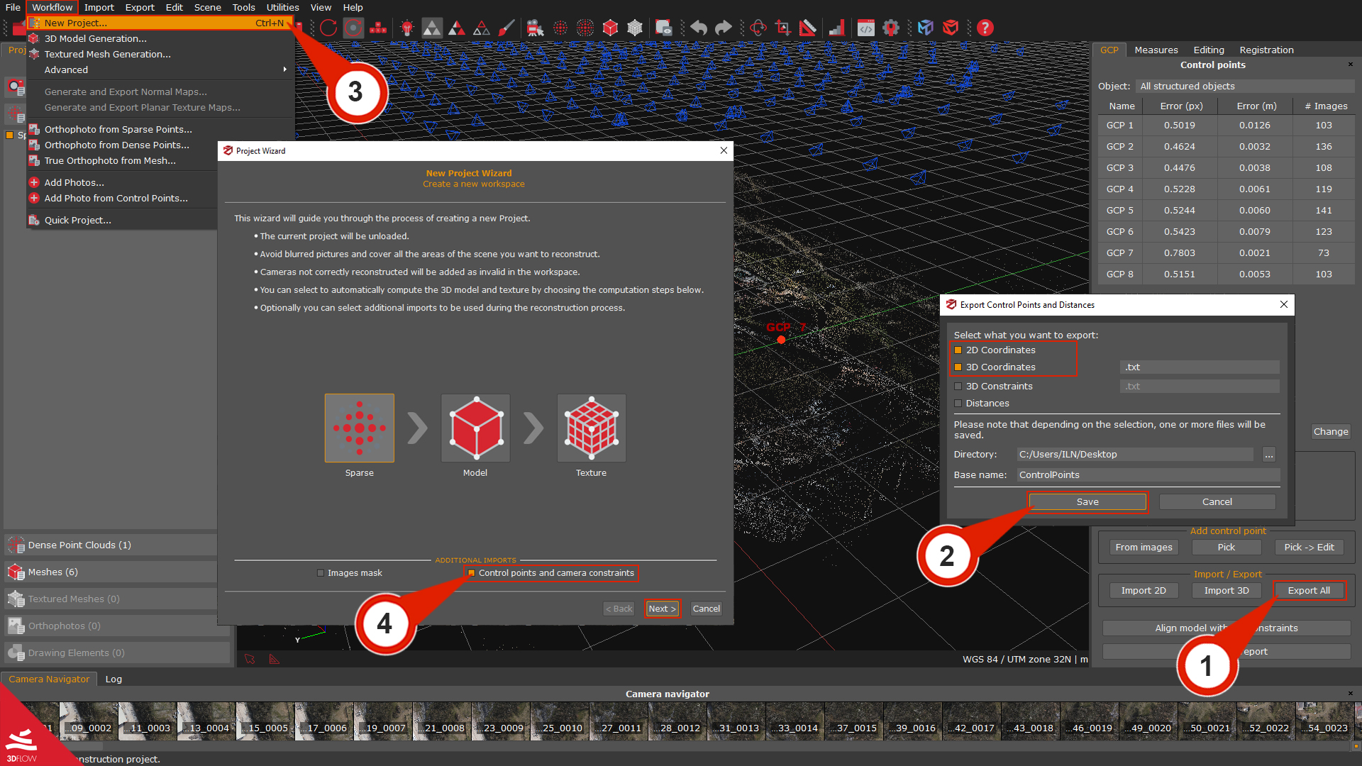
After importing the 3D coordinates and adding them as 2D coordinates in the images, you need to click the “Export All” (1) button in the GCP panel. This action will open the Export Control Points and Distances window. Make sure to check the flags for both 2D coordinates and 3D coordinates. Then, select the desired directory and provide a file name, and finally, click the “Save”(2) button.
Please, navigate the Workflow menu and select the “New project” (3) option for launching the New Project Wizard. Ensure that the “Control points camera constraints” (4) checkbox is activated on the first page before proceeding.
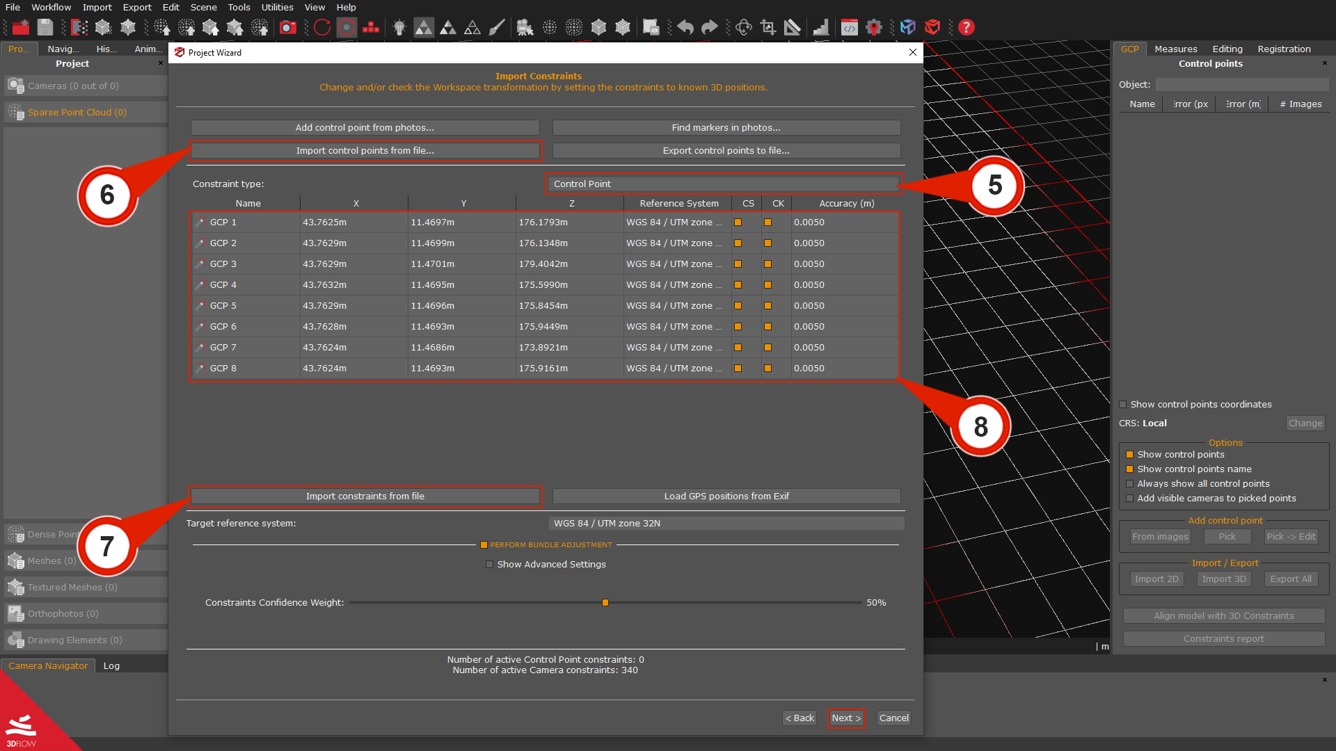
In the Import constraint page, change the Constraint type filter to “Control Point” (5). Then, press the “Import control points from file” (6) button to import the previously exported 2D coordinates file. Finally, click the “Import constraints from the file” (7) button to import the exported file with 3D spatial coordinates.
All the GCPs with their associated 3D spatial coordinates (8) will be listed in the center of the Import constraint window. At this stage, you can change the Target reference system and assign Constraint or Checkpoint statuses to each point. Once ready, click “Next” to proceed and start the reconstruction.
Scaling and georeferencing the model with 3D constraints
The 3D reconstruction is up to an arbitrary scale, rotation, and translation in 3DF Zephyr. Whether you have manually added GCPs to the Zephyr project or imported control points from an external file, it is possible to associate them with the world spatial coordinates for scaling and georeferencing the project.
As a rule of thumb:
- – using 1 control point will translate the world;
– using 2 control points will translate the world and set a global scale;
– using 3 or more control points will set a full transformation that will scale, translate and rotate the world (georeferencing process).
Note: the coordinates you are importing and the GCPs you have added to the project must have the same name/label.
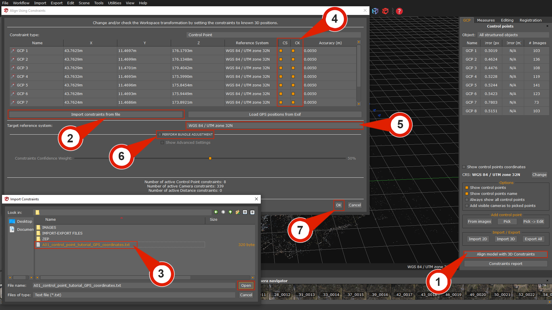
Press the “Align model with 3D Constraint” (1) button in the GCP panel. In the Align using constraint window, click the “Import constraints from file (2)” button to browse the external file located in the sample dataset linked above and named A01_control_point_tutorial_GPS_coordinates.txt (3) and click the “Open” button. You can skip points (2) and (3) if you have followed the above-described Method 3: importing control points from a text file in Zephyr.
You will notice that both the Constraint and Check columns will be enabled for each control point by default, and if you are working with RTK data, these columns will be enabled for each camera position.

Difference between Constraints and Checkpoints
Constraints are the most confident points in terms of accuracy level, and 3DF Zephyr relies on them to drive the scaling process.
Checkpoints are references that the software only considers while scaling to keep the error value monitored.
Example:Let’s think about an aerial survey where you have both coordinates taken using the drone’s GPS system and coordinates taken on the ground with a total station, for instance. Once you have placed your points in 3DF Zephyr, you can choose which points must be the Constraints, namely the points you are confident (of their accuracy) the most, and which points will be taken into account as simple references to keep the error value monitored (Checkpoints).
Once you have selected your Constraints and Checkpoints (4), you can deal with the input and target reference system (5) settings.
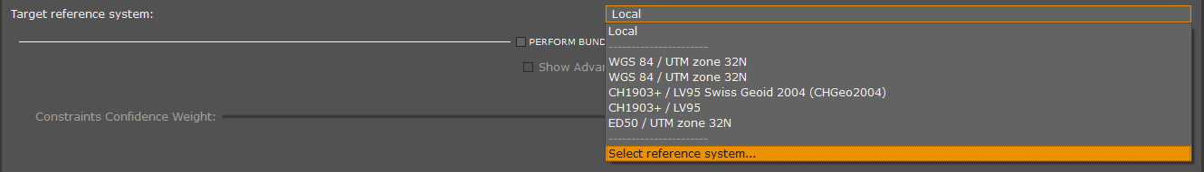
You can set both the input/target reference system and the Geoid Gravity Model. Click the “Select Reference System” option to open the Coordinate system database:
The Projection Coordinates System window will open:
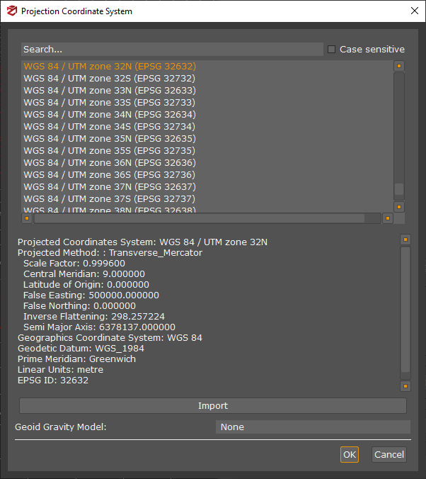
Select a Coordinate system from the database list, type its name or EPSG code, or import a new one from an external source by clicking the “Import” button.
A Geoid Gravity Model can also be downloaded and loaded in relation to the Coordinate Reference System. Following this link, you can download some of the most commonly used Geoids: https://www.3dflow.net/geoids/. Click the “Ok” button when you are set.
Last, you can enable/disable the “Perform Bundle Adjustment” (6) option to optimize the camera positions minimizing the reprojection error of the control points you have added to the project. For more details, see the tutorial dedicated to Bundle Adjustment.
Once you are set, click the “OK” (7) button to run the scaling/georeferencing process. An error report will appear when the process is finished, and you can always call it back by clicking on Tools > Control points > Show alignment info.
Scaling using distances
In 3DF Zephyr can use an alternative method for scaling the project with known distances.
Control distances can be defined as the distance between two control points, between a control point and a camera, or between two cameras.
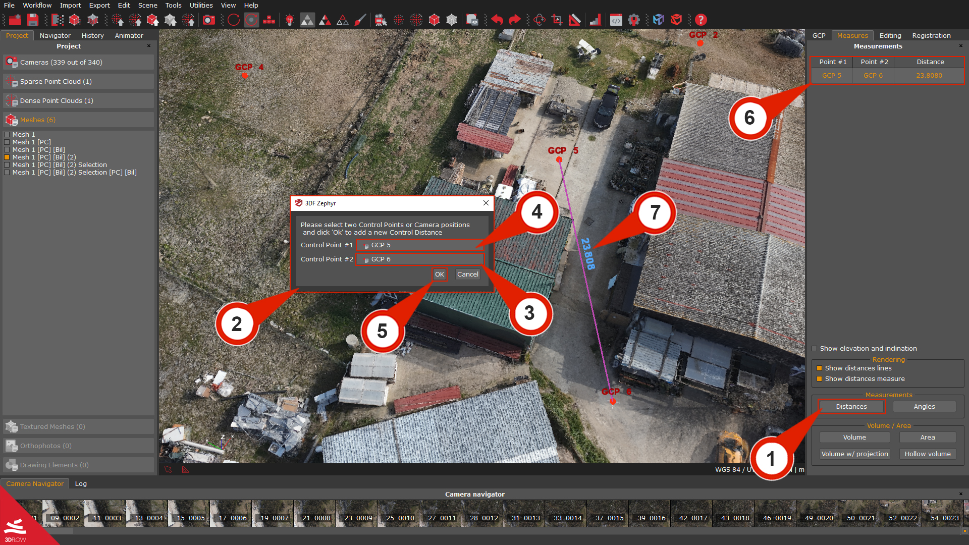
Click on the “Distance” (1) button in the Measures tab, and the Control point selection window (2) will pop up. Pick the two control points from this window from the Control Point #1 selection menu (3) and the Control Point #2 selection menu (4).
This example shows two control points (GCP 5 and GCP 6), which can also be cameras. Once you click “OK” (5), the control points and distance will also appear in the Control Distance List (6), and the distance will be drawn as a colored line (7) and rendered onto the screen (the distance in this example is 23.808 meters)
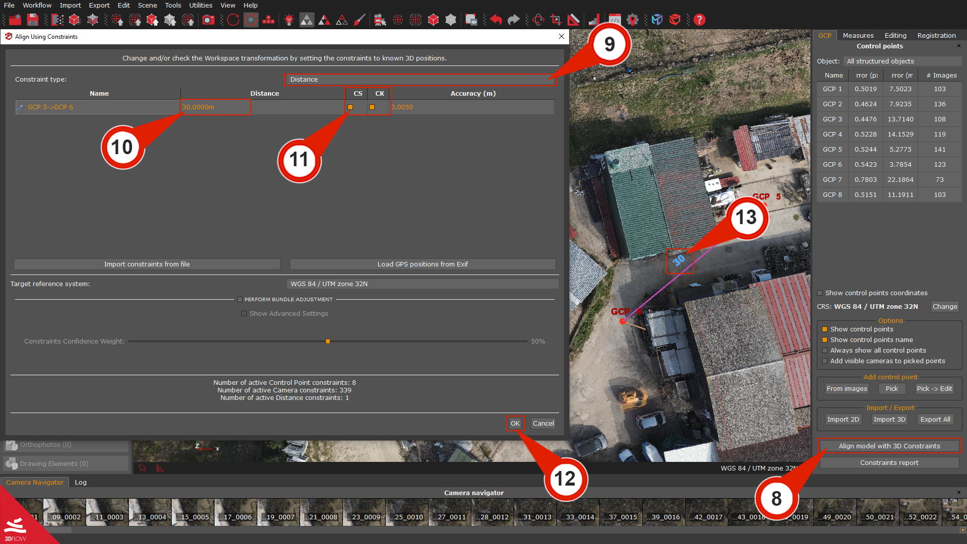
To Scale the world using Control distances, simply click on the “Align model with 3D Constraint” (8) button in the GCP panel, and the Align using constraints window will appear.
Click on the Constraint type menu and select “Distance” (9), to view the previously created measure, you can set the desired “Distance value” (10) by clicking on the distance column; for example, you can set it to 30.000 meters.
You can flag the previously created control distance(s) as Constraint and/or Check (11) as before with the Control points and then click the “OK”(12) button.
You’re done! The whole mesh will be scaled on the newly inserted value (13).