Tutorial #A12 : Multiband dataset processing tutorial
Multiband datasets
Welcome to the 3DF Zephyr tutorial series.
In this tutorial, you will learn how to process multiband datasets and calibrate multispectral images from Rededge Micasense Cameras.
This tutorial cannot be completed with 3DF Zephyr Free or Lite versions!
Summary
Introduction
3DF Zephyr supports multispectral image datasets from different devices; it can automatically read the band information in the tiff metadata, recognize them as layers, and add them to the New Project Wizard. It’s possible to select the main layer that will be used for the Structure from the Motion phase and the other secondary layers that can be switched as necessary.
The following Step 1 – The Multispectral images Calibration section is not mandatory, and it will describe the process of converting raw multispectral images to radiometrically calibrated reflectance images. Zephyr will automatically create layers based on the tiff metadata, and the resulting calibrated images will be renamed with the corresponding band abbreviation.
For example, filename_1.jpg and filename_2.jpg are two bands (1,2) of the same photo “filename“.
After the calibration process, the images will be renamed: filename_REG.jpg and filename_GRE.jpg.
Note: currently supported sensors for the calibration process are: MicaSense Altum, MicaSense RedEdge-S, MicaSense RedEdg-M, and RedEdge-P.
If you don’t need to calibrate your camera, you can skip directly to Step 2 – Creating a new multiband project.
The following dataset created with the RedEdge Camera by MicaSense will be used as an example. Please click on this link for download:
 | Download RedEdge Sample Data of MicaSense |
Step 1 – The calibration of multispectral images
In order to calibrate your dataset made with a RedEdge camera, you need to take one photo of the Calibrated Reflectance Panel (CRP). In the case of the provided sample dataset for this tutorial, 5 images of the CRP can be used, which are numbered 1, 2, 3, 4, and 5, corresponding to the G, B, R, NIR, and GRE bands.
Note:Newer sensors can produce 6 or more bands depending on the model.
From the “Utilities” menu, select “Multispectral” and then “Launch multispectral calibration“. The Radiometric calibration wizard will appear. Click the “Next” button to proceed.
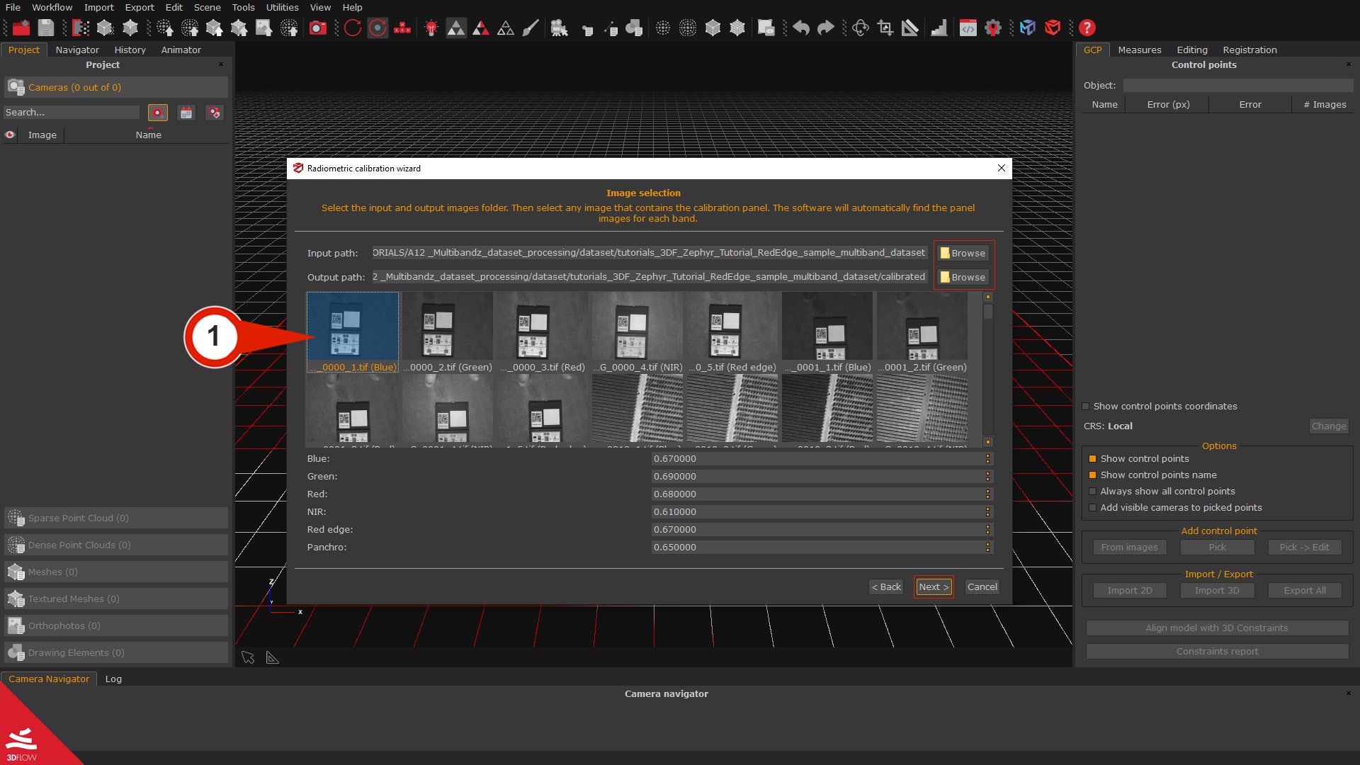
On the Image Selection page, navigate to select the directory for your dataset’s Input path and the directory for the Output path where the calibrated images will be saved. It is recommended to use a distinct output directory (for example, a newly created folder named “calibrated”) to maintain a clear and organized workflow.
The normalization values for the bands can be inserted in the page’s lower part. Utilizing the default values provided by Zephyr will allow you to proceed, but it’s suggested to use the values provided by the CRP manufacturer to improve the calibration.
To finalize this step, choose the best capture of the Calibration panel (1) and then click on the “Next” button.
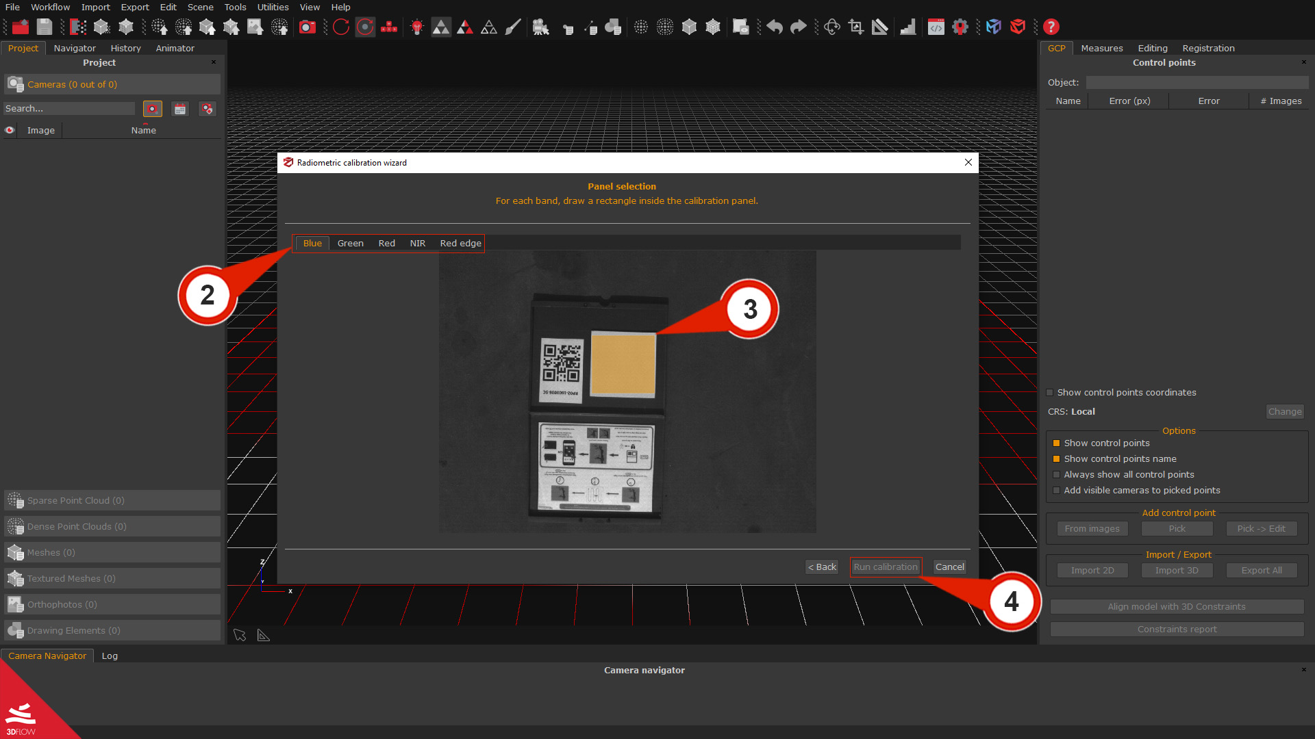
In the Panel Selection page, each detected band is grouped in tabs (2). A yellow rectangle (3) should be drawn by holding down and dragging the left mouse button in the white square area of the panel. Please ensure that the rectangle is only drawn over the white inside part of the square.
Once you have repeated this step for all five bands, the Run Calibration (4) button will be enabled, and it will be possible to click it to run the calibration.
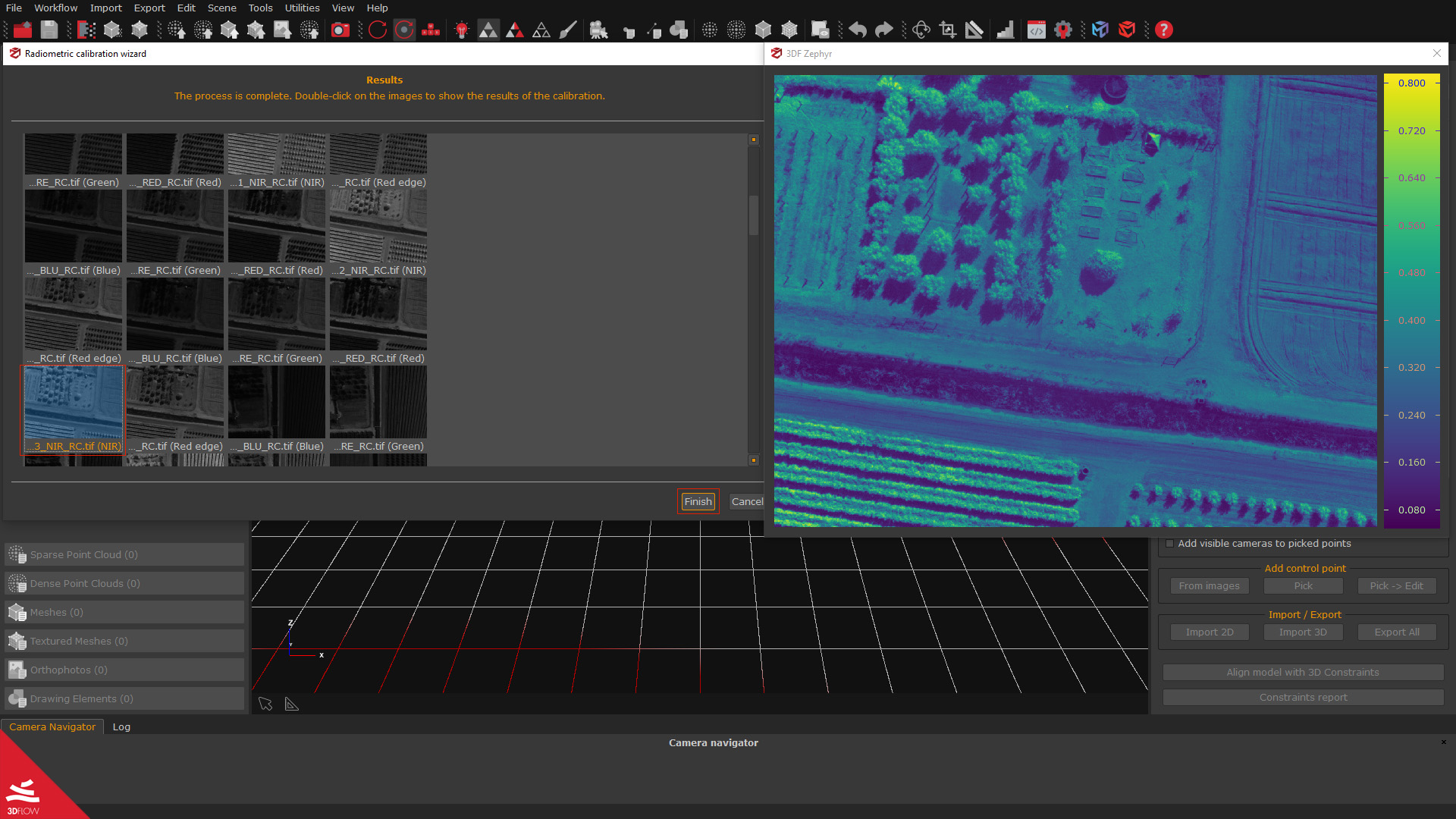
After completing the elaboration process, the wizard’s Results page will display calibrated images for each band. Users can either double-click on any image to view it or click the “Finish” button to conclude the calibration.
Step 2 – Creating a new multiband project
To create a multiband project in Zephyr, launch the New project wizard and incorporate the calibrated images into the workflow. Panel images are not required as they have already been processed during the calibration stage. Zephyr will automatically identify multiple layers if the image filenames have appropriate suffixes:
filename_1.jpg and filename_2.jpg can be considered as two bands (1, 2) of the same photo “filename”.
After that, the wizard will ask you if you wish to create multiple layers.
– If you press the “YES”button, Zephyr will automatically split the files into an appropriate number of layers according to the suffix.
– If you press the “NO” button, it will still possible to create layers by right-clicking and selecting “Add layer“ option later.
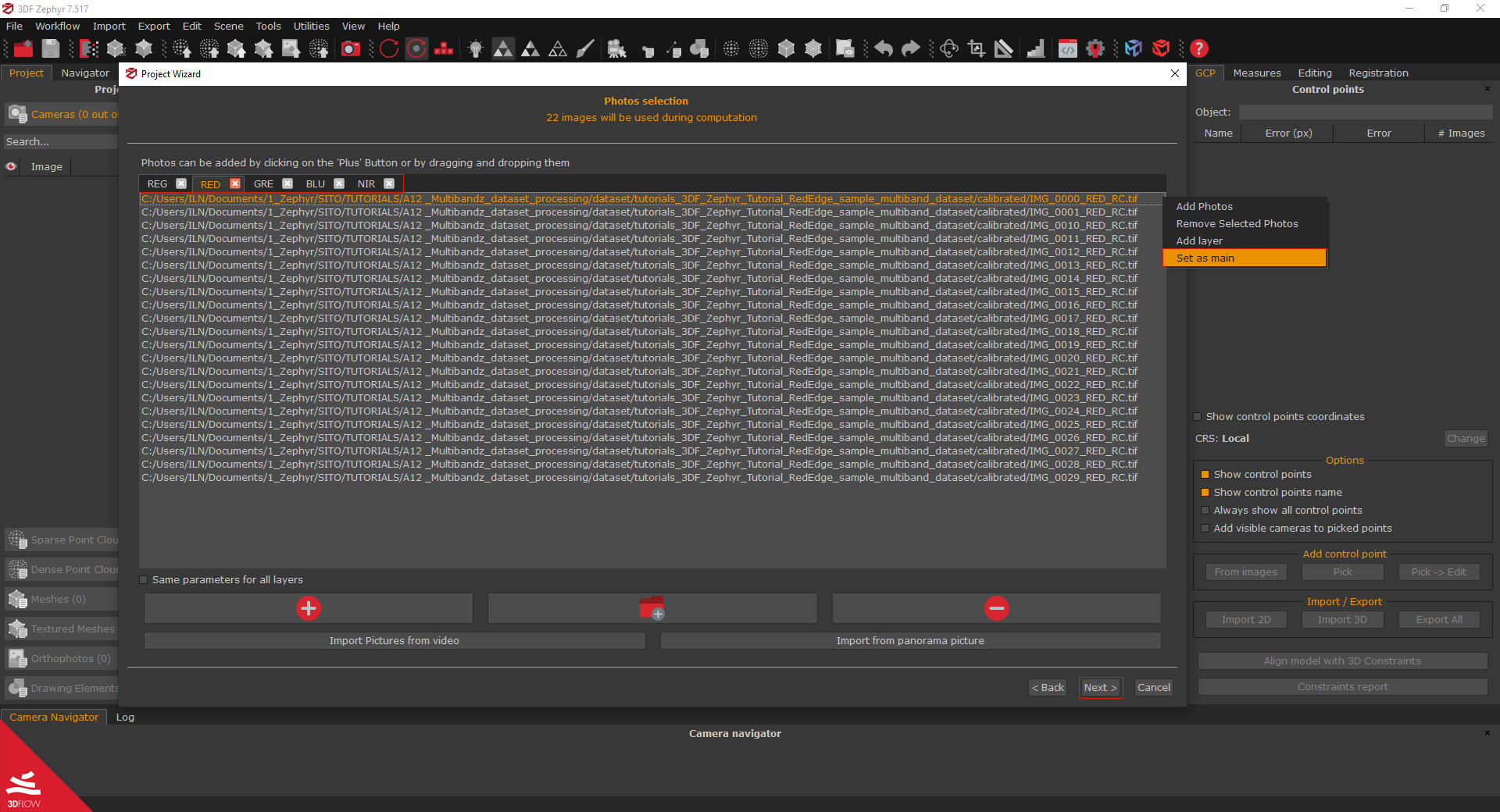
Layers will be automatically organized into bands according to the image suffixes. Zephyr will detect the main band automatically. In this case, when utilizing the provided tutorial’s dataset and following the Step 1 – The calibration of multispectral images, the REG band will be identified and showcased as the leftmost tab by default.
To modify the main layer, simply right-click on the image list within the appropriate tab and choose “Set as main“.
Clicking the “Next” button will navigate to the standard reconstruction workflow. Please select the suitable reconstruction options for your dataset and advance through the pages of the New project wizard using the “Next” button. On the final page, initiate the reconstruction by clicking the “Run” button.
Update the project with multispectral colors
When you reconstruct a multispectral dataset, you get a grayscale mesh by default, because the images for the various bands are visualized in grayscale color. Either the point clouds or meshes can have their colors upgraded by right-clicking on the point cloud or Mesh in the Project panel and selecting the Filters and “Update colors” option. It’s also possible to launch the Update colors wizard from the right panel Editing and the “Update colors” button.
In the Update color window it’s possible to select the “Model” and the color “Mode”.
Since you are working with a multispectral project, only these two relative functions of updating the colors will be described:
Mode by bands Combination
By setting a mathematical formula in the Combine Layer dialog,each point/triangle of the point cloud/mesh is updated with the calculated colormap. This mode is used if you want to display, for example, the NDVI index directly on the mesh or cloud of points. It’s possible to save or load the created formulas to use them later by clicking on the “Save” or “Load” buttons.
Mode by bands to RGB
This mode is employed to color the mesh as expected in RGB colors. By default, it automatically assigns each band to its corresponding color channel (e.g., the red band to the red color channel). However, you can still adjust the order of the bands as required.
Step 3 – The multispectral orthophoto generation process
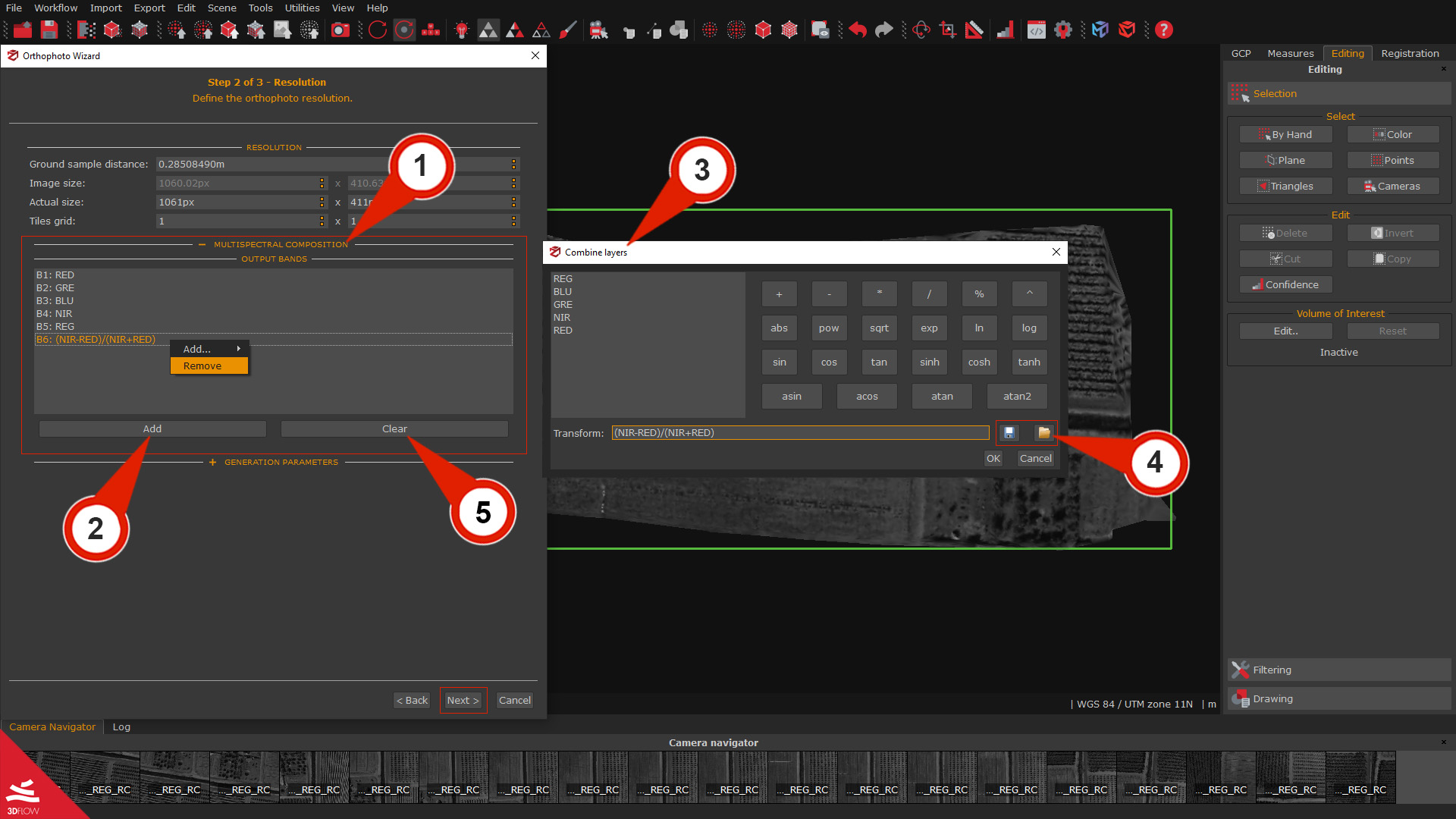
The multi-band information stored in the workspace is utilized for further processing within 3DF Zephyr. In the “Step 2 – Resolution” page of the Orthophoto generation tutorial, the software automatically displays the found Output bands (1) and the NDVI index is automatically added (if possible). For example, in this tutorial, the RED, GRE, BLU, NIR, REG, and NDVI are added in the orthophoto selection box.
Users can customize the combination of output bands by selecting “Add band” (2) and defining a mathematical formula in the “Combine Layer” (3) dialog. This customization facilitates the combination and display of different bands in the orthophoto. Additionally, users can Save or Load (4) created formulas for future use by clicking the respective buttons in the dialog. To remove all bands, users can click the “Clear” (5) button. Alternatively, to delete a specific band, users can right-click on it and select “Remove”.
When all the bands are set, click on the “Next” button for proceed with the Orthophoto Generation wizard.
The NDVI (Normalized Difference Vegetation Index) band is a index in remote sensing for assessing the health and coverage of vegetation in a given area. It’s derived from the normalized difference between near-infrared reflectance (NIR) and red band reflectance (RED) across the electromagnetic spectrum. The NDVI index offers insights into vegetation quantity and density, with higher values suggesting more vegetative growth.
Below a a transformation formula example for NDVI calculation:
(a-b)/(a+b)
(NIR-RED)/(NIR+RED)
Note: to load the NDVI formula example, click on the Load Transform button, select NDVI and then “OK”.
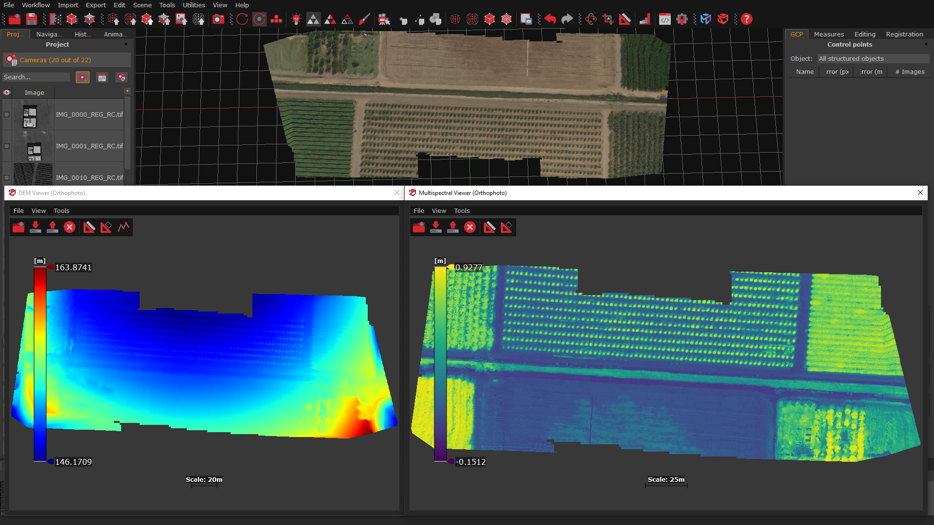
[/spoiler]At the end of the process, Zephyr will show the orthophoto in the DEM viewer and the Multispectral viewer with the bands set during the workflow.
Save the multi-band orthophoto on the computer
At the end of the generation process, the new multi-band orthophoto will be listed in the Project tab under the section Orthophoto.
By right-clicking on the orthophoto will be possible to choose the option “Export” (1), and the Export orthophoto (2) window will appear. It’s possible to choose different export settings; see the description below:
The Export (3) drop-down menu offers the option to export only the orthophoto, the DSM, DTM, or all the files.
The Image format (4) drop-down menu allows you to save the Multi-band Orthophoto in *.tifformat.
As additional export options, the following check-boxes will allow you to export additional file formats or the images in separate bands:
- – Export each band separately: exports the orthophoto’s bands in separate image files.
– Export World file: exports the orthophoto in World file format.
The Tiff pyramids level parameter will allow storing inside the generated Tiff orthophoto a pyramids levels layers, which can improve the display of raster data by retrieving only data at a specific resolution required for display.
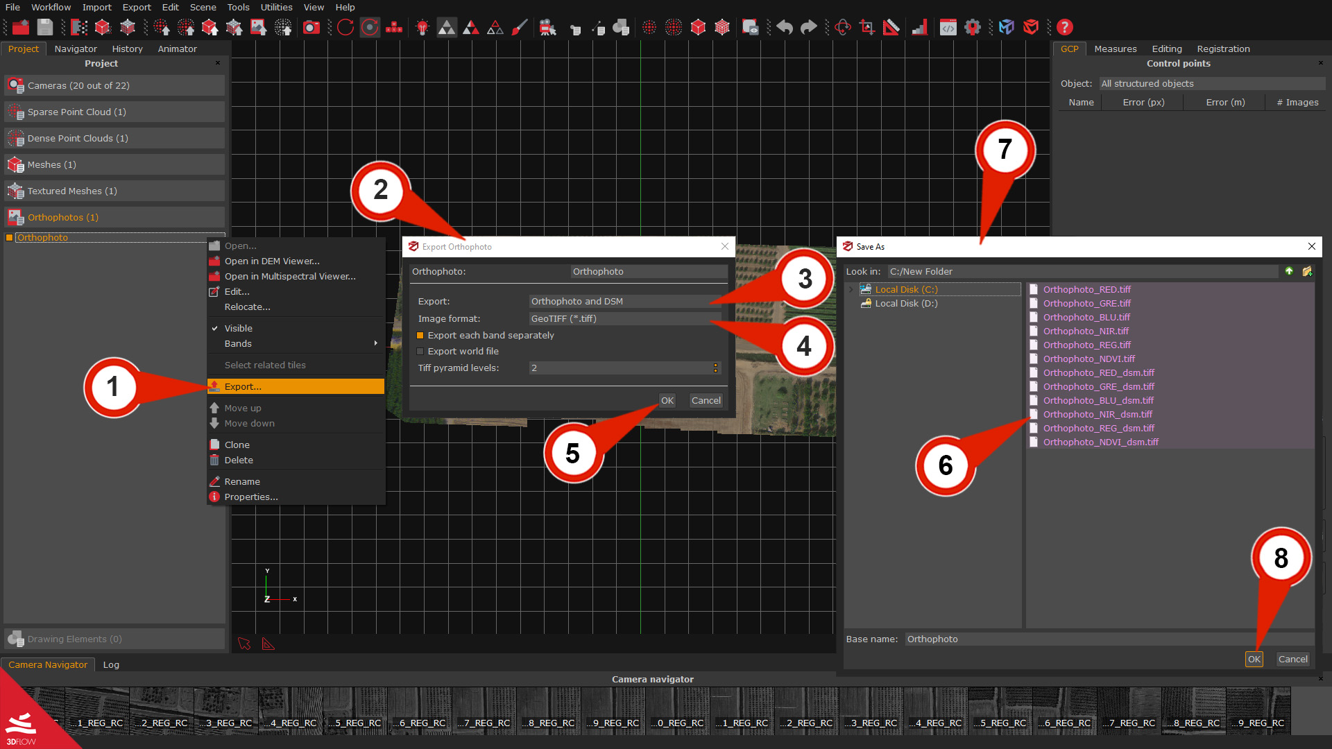
After establishing the parameters for saving the orthophoto, click “OK”(5). A preview (6) of the exported files will be shown in the Save As (7) window; select the file name and destination folder, and then the “OK”(8) button to save.
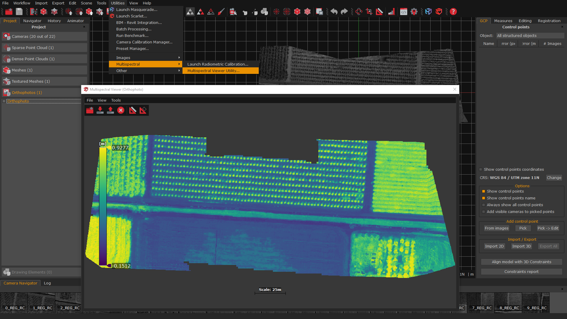
Step 4 – The multispectral viewer utility
Similarly to the DEM viewer, generated orthophoto can be viewed directly in 3DF Zephyr in the included Multispectral viewer utility with the multi bands colors applied.
The viewer can be opened from the menu Utilities > Multispectral > Multispectral viewer utility.
Note: the Multispectral viewer utility can be open directly from the Project tab and right-clicking on the multi-band orthophoto.
In The File menu, you can use the following options to load the images in the viewer:
- – Open from files option: allow to load tag images in .tif format. This command is useful to open and check even those files that are not necessarily related to the project you are working on.
– Open from workspace option: it loads the multi-band orthophoto previously saved in the current project.
– Export color images option: it allows exporting multi-band orthophoto to one of the following image formats: .png, .jpg, .bmp.
In the View menu it’s possible to set different color options for visualizing the orthophoto and it’s bands:
- – Band option: it allows to change the orthophoto’s bands visualized in the viewer.
– Colormap option: it allow to set the orthophoto’s colormap in the viewer. The default colormap is viridis, but it can be changed by clicking on it. The Invert option will invert the colors and with Set color map levels a different numbers of level can be inserted.
The Tools menu offers the possibility to make measurements on the multiband orthophoto:
- – The Enable distance tool: it allows you to define and measure distances.
– The Enable area tool: it allows you to place (at least) 3 points and calculate an area.
The Color bar on the left side of the viewer allows you to set the elevation range thanks to the minimum and maximum elevation thresholds.
Please, move the slider to the left/right to see the difference of the color bar range sets.

