Tutorial #01 : How to convert photos in 3D models with 3DF Zephyr
Getting started with 3DF Zephyr
Welcome to the 3DF Zephyr tutorial series. In this tutorial, you will learn the basic steps for turning pictures into 3D models with 3DF Zephyr.
IMPORTANT NOTE: The images in the following tutorial describe the full version of 3DF Zephyr, showcasing all its features. Please note that 3DF Zephyr Free and 3DF Zephyr Lite follow the same workflow for 3D reconstruction, but not all options may be available. You can consult the 3DF Zephyr Feature Comparison page to view the available features list for each version.
Summary
Introduction
Creating 3D models from pictures in Zephyr requires a dataset of images taken using photogrammetry techniques. You can use your pictures by following this tutorial. Please refer to these base guidelines to learn the best practices for acquiring a photogrammetry dataset. Note that the image acquisition phase is crucial for successful photogrammetry reconstruction.
NOTE: before you start a photogrammetry reconstruction in 3DF Zephyr, it’s important to use a reliable image dataset as input. Please avoid using blurred images and datasets with no overlapping pictures, as these can result in poor-quality reconstructions. Also, never crop, cut, or edit the pictures in Photoshop or any other image editing software.
A sample dataset can be used for training purposes in this tutorial. Please download and extract the “Dataset – Cherub” zip file on your computer. This dataset consists of 65 photos. For users of 3DF Zephyr Free, which is limited to 50 photos, select the first 50 photos only.
 | Download Dataset – Cherub (531MB) |
 | Download – Cherub .ZEP file (340MB) |
The following links are available for downloading and installing the suitable version of 3DF Zephyr to start the tutorial:
Step 1 – Creating a new project
Starting the new project wizard
To create a new project, click on “Workflow” > “New Project” (1). The Project Wizard (2) will guide through the picture import and camera orientation phase setup. It’s possible to select the required 3D reconstruction phase(s) in addition to the camera orientation phase by enabling the corresponding icons in the Computation phases graph (3).
- SPARSE: This option will orient the images and generate a Sparse point cloud.
- MODEL: This option will create the Sparse point cloud, Dense point cloud, and Mesh.
- TEXTURE: This option will include all the previous 3D products and generate a Mesh with texture.
Depending on the version of Zephyr used, the Additional option (4) section can include the following check-boxes: Import of image masks, Define constraints (2D and 3D coordinates), and Setup of multi-camera groups. If the additional options are unnecessary, click the “Next” button to proceed through the wizard.
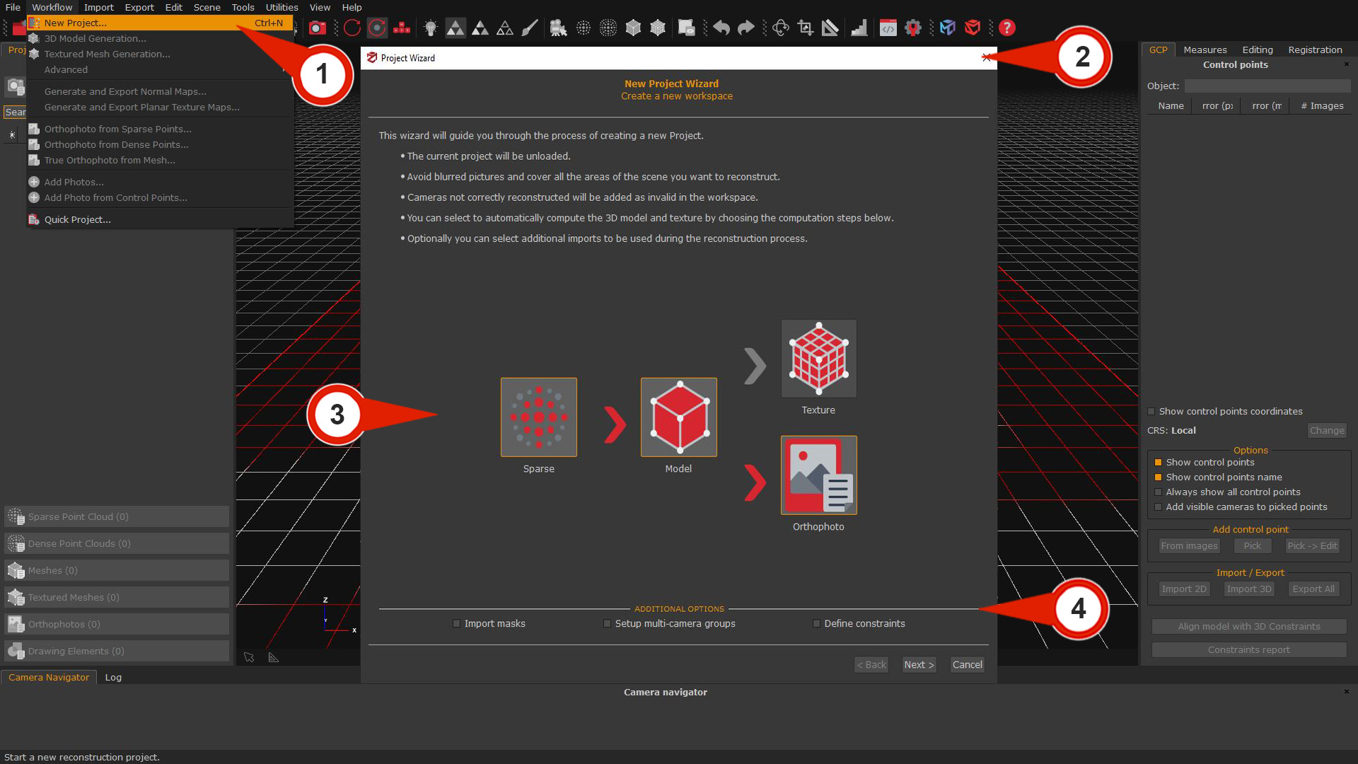
Note: only in 3DF Zephyr Full version, it’s possible to decide in the final phase to generate an Orthophoto on the Z axis along with the Mesh with texture. Please, follow this link: Section A: Generating orthophoto via new project wizard for the advanced orthophoto workflow.
Selecting the images
The upcoming window will present the Photo selection page, providing the ability to include images in the process via Zephyr.
Click on the “Add directory” (5) button, browse to the directory where your dataset is located, and then press the “Select folder” button. If there are sub-directories in the folder, Zephyr will prompt you with a pop-up window to include them in the wizard by clicking a “YES” or “NO” button. You can also drag and drop images or folders directly into the Photo selection space.
Alternatively, you can click the Add images (6) button, browse to the directory where your dataset is located, select all the previously extracted images, and then click the “Open” button. If needed, you can select one or all images (ctrl+a) and click the “Remove” (7) button to exclude them from the workflow.
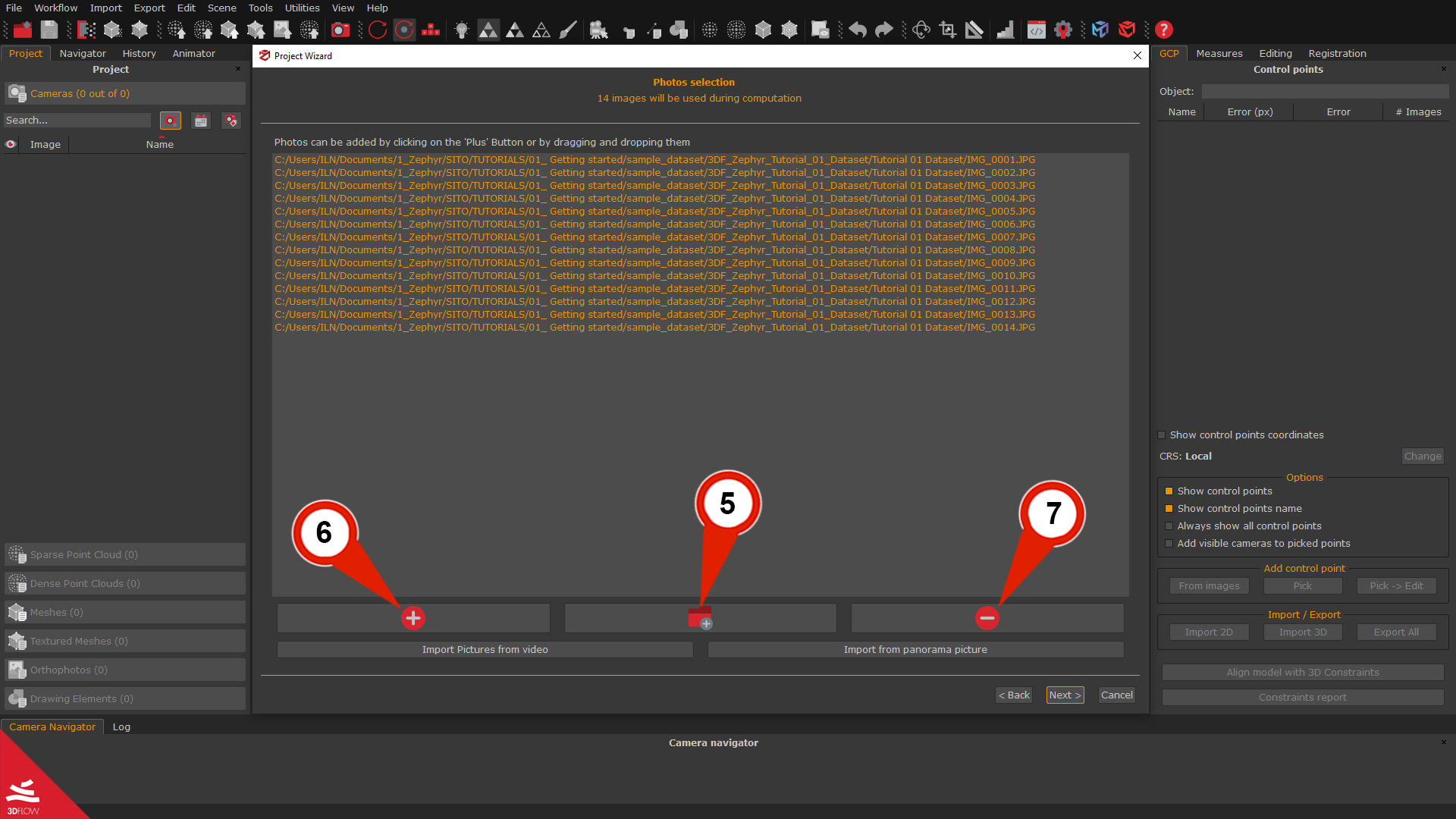
Most datasets are usually created using .JPG or .PNG files, but Zephyr can also use many other image formats, such as rawNEF, CR2, ARW2, etc.). When all the pictures are selected, press the “Next” button to proceed to the following wizard page.
Camera calibration overview
Once the images to be processed are loaded the Camera Calibration page will be available. 3DF Zephyr will automatically retrieve the camera calibration parameters and assign them to the pictures. It’s still possible to Add a New Calibration or Modify the Calibration but it’s advised for expert users only for particular purposes.
The interface will display a list of the imported pictures along with their calibration summary, which 3DF Zephyr and its Structure from Motion algorithm will specifically use. 3DF Zephyr can download pre-calibrated camera parameters to speed up the processing when connected to the internet. However, the software is fully auto-calibrated, allowing it to function offline, and in most cases, all the parameters can be left as default.
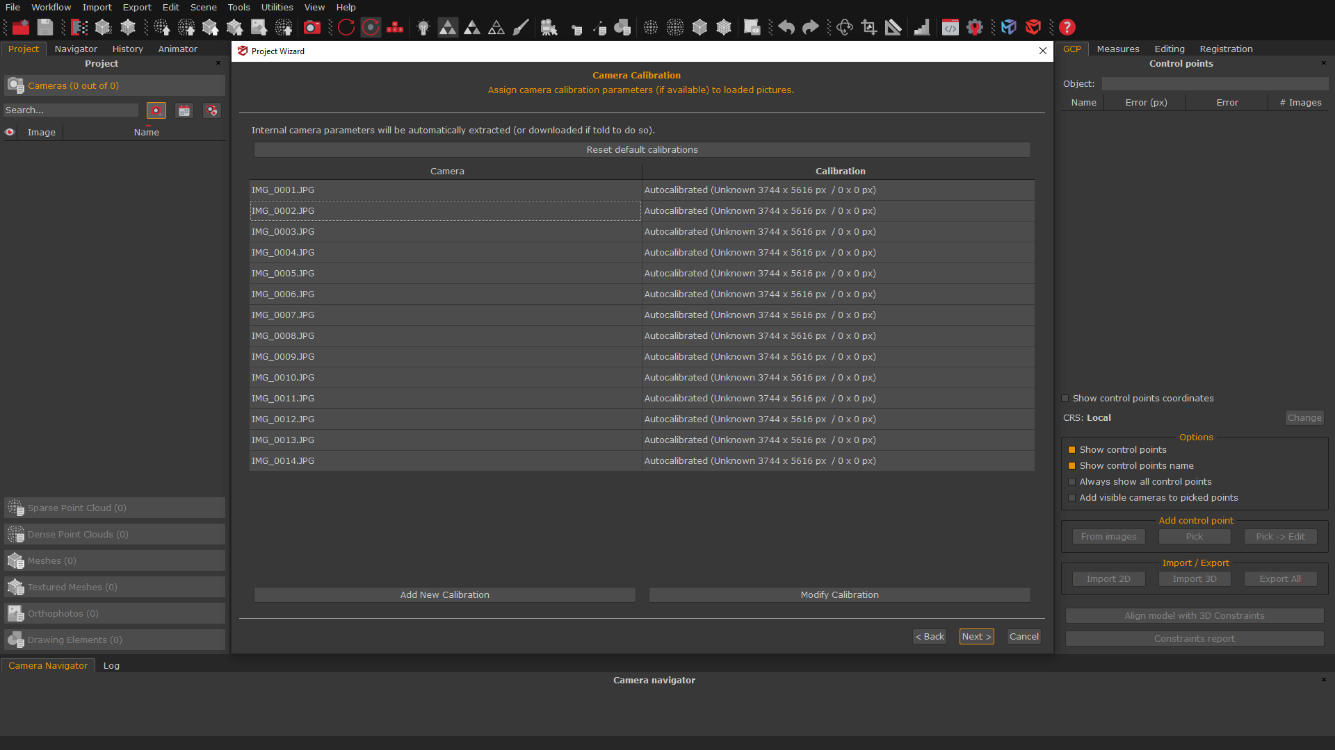
Click the “Next” button to proceed to Step 2: Configure the reconstruction settings.
Step 2 – Configure the reconstruction settings
In this tutorial step, the settings pages of 3DF Zephyr will be illustrated. The related settings pages will consistently appear depending on the 3D reconstruction phase(s) chosen in step 1.
Camera orientation and sparse point cloud generation
The first phase of 3D reconstruction is called Structure from Motion and results in a Sparse point cloud. Zephyr analyzes each image, identifies its features, and compares each image with a subset of the other pictures. This process determines the correct positions and orientations of each photo loaded into Zephyr.
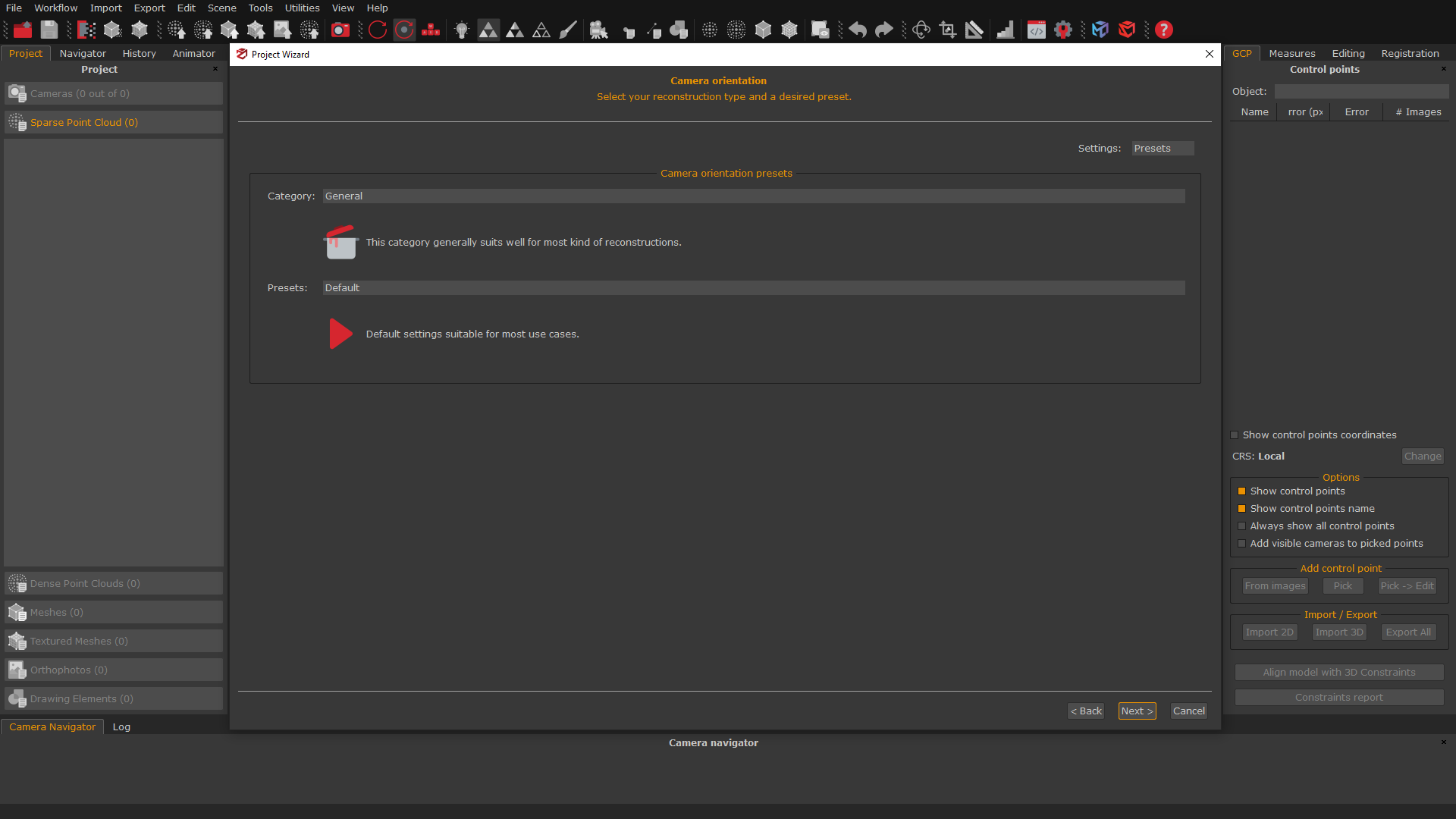
In the Camera orientation page, users should define settings Category depending on the captured scenario or subject.
| CATEGORY NAME | DESCRIPTION | |
 | General | This settings category is applicable to a wide range of scenarios. It is particularly effective for small objects within close-range datasets and is recommended for uncertain situations concerning the appropriate category to select. |
 | Aerial – Nadiral images | This settings category is useful for reconstructing top-down view scenarios, typically with UAV datasets. |
 | Urban | This settings category can be selected when photos are taken from varying distances or if different types of photos are mixed. It could be useful when the subjects are buildings, facades, or scenarios shots in urban environment. |
 | Human Body | This settings category is ideal for scanning human body parts, including close-ups or full figures. |
 | Surface Scan | This settings category is useful to reconstruct flat surface close-ups, such as terrain or ground. |
 | Vertical Structure | This settings category is best for reconstructing thin vertical structures, like telecommunication towers, from UAV pictures. |
Selecting the Preset option is also fundamental for proceeding and must be chosen according to the desired accuracy and quality level decided for the 3D model reconstruction. The following three options are available:
| PRESET NAME | DESCRIPTION | |
 | Fast | This preset reduces processing times by lowering the resolution, decreasing bundle adjustment iterations, and reducing the number of key points. It’s useful for quick tests to determine if additional images are needed in the survey. |
 | Default | This preset is suitable for use in a wide range of scenarios. |
 | Deep | This preset increases the bundle adjustment iterations, the number of key points, and camera matches. It can be used when cameras are loosed in the default settings mode. |
The resulting Oriented cameras and Sparse point cloud will be listed in the left Project tab. Click the “Next” button for proceeding to the Dense point cloud creation page.
Dense point cloud generation
The Zephyr Multiview stereo algorithm can extract accurate Dense point clouds from a dataset of 2D images by matching the pixels between the pictures.
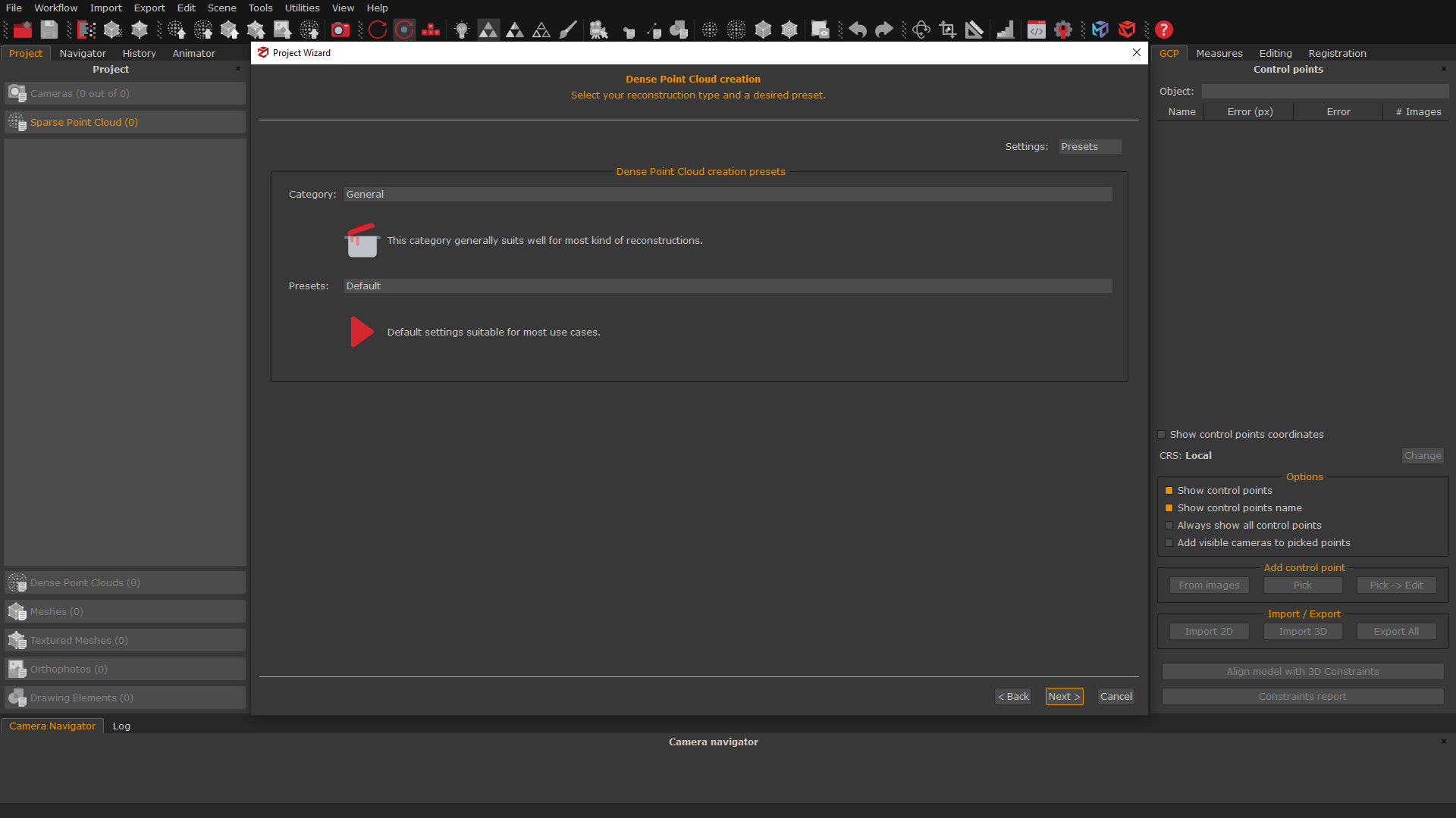
In the Dense point cloud creation page, users should define settings Category depending on the scenario/subject they have captured:
Note: keeping the Dense point cloud category used in the previous Camera orientation stage is highly recommended.
| CATEGORY NAME | DESCRIPTION | |
| General | This settings category is suitable for most situations, particularly for small objects in close-range datasets, and it is an ideal choice when there is uncertainty surrounding the selection of a category. |
| Aerial – Nadiral images | This settings category is useful for reconstructing top-down view scenarios, typically with UAV datasets. |
| Urban | This settings category can be selected when photos are taken from varying distances or if different types of photos are mixed. It could be useful when the subject are buildings, facades or scenarios that are shots in urban environment. |
| Human Body | This settings category is ideal for scanning human body parts, including close-ups or full figures. |
| Surface Scan | This settings category is useful to reconstruct flat surface close-ups, such as terrain or ground. |
| Vertical Structure | This settings category is best for reconstructing thin vertical structures, like telecommunication towers, from UAV pictures. |
Selecting the Preset option is fundamental for proceeding and must be chosen according to the desired accuracy and quality level decided for the 3D model reconstruction. The following three options are available:
| PRESET NAME | DESCRIPTION | |
| Preview | This preset allows to skip the stereo phase and use the Sparse point cloud. |
| Default | This preset can be used in most of the cases. |
| High details | this preset increases the settings beyond the default one, resulting in a richer and denser point cloud. |
After processing, the resulting Dense point cloud will be available in the left Project tab of the Zephyr’s interface. To proceed to the following page, click on the “Next” button once again.
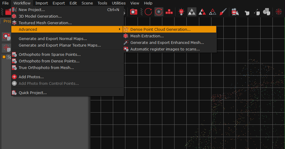
The Dense point cloud creation phase can be initiated independently from the New project creation process within the Zephyr workspace by navigating through the Workflow > Advanced > Dense point cloud generation menus. This phase requires that Oriented cameras and a Sparse point cloud have already been created and are listed in the Project tab.
Mesh extraction
The Zephyr Mesh extraction algorithm will generate a Mesh from the Dense point cloud.

The Mesh generation categories on the Surface Reconstruction page should also be chosen depending on the scenario.
Note: it is highly recommended to use the same Mesh settings category used in the previous Dense Point Cloud creation phase.
| CATEGORY NAME | DESCRIPTION | |
| General | This settings category is suitable for most situations, particularly for small objects in close-range datasets, and it is an ideal choice when there is uncertainty surrounding the selection of a category. |
| Aerial – Nadiral images | This settings category is useful for reconstructing top-down view scenarios, typically with UAV datasets. |
| Urban | This settings category can be selected when photos are taken from varying distances or if different types of photos are mixed. I could be useful when the subject are buildings, facades, or scenarios shots in an urban environment. |
| Human Body | This settings category is ideal for scanning human body parts, including close-ups or full figures. |
| Surface Scan | This settings category is useful to reconstruct flat surface close-ups, such as terrain or ground. |
| Vertical Structure | This settings category is best for reconstructing thin vertical structures, like telecommunication towers, from UAV pictures. |
 | Laser scan | This settings category is designed to extract meshes from laser scans point clouds. |
Selecting the Preset option is fundamental for proceeding and must be chosen according to the desired accuracy and quality level decided for the 3D model reconstruction. The following three options are available:
| PRESET NAME | DESCRIPTION | |
| Preview | This preset has settings similar to the Default preset but disables the Photoconsistency optimization algorithm. |
| Default | This preset can be used in most of the cases. |
| High details | This preset has an increased resolution during the Photoconsistency optimization than the default one. It allows producing a mesh with more polygons and details, but requires more time. |
The resulting Mesh will be listed in the left Project tab. Click again the “Next” button to proceed to the following page.
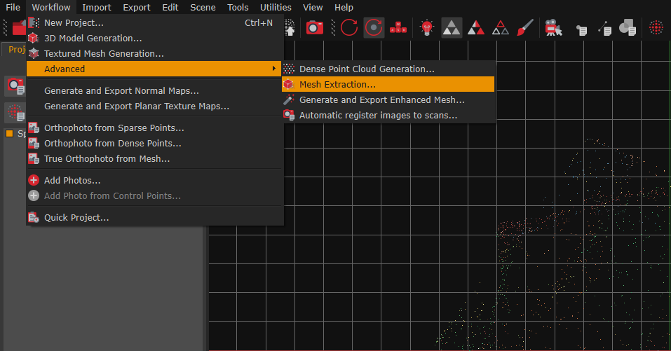
The Mesh Extraction phase can be initiated independently from the New project creation process within the Zephyr workspace, by navigating through the Workflow > Advanced > Mesh extraction menus. This phase requires a Dense Point Cloud created and listed in the Project tab.
Textured mesh generation
In this last phase, the Zephyr’s Texturing algorithm will deal with the image’s color balance and generate a suitable Texture for the mesh.
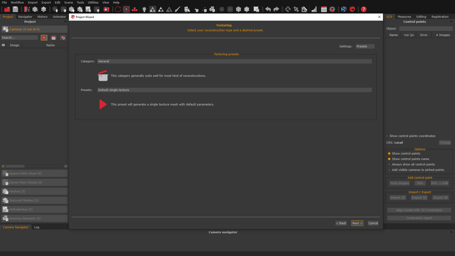
In the Texturing settings page, the Texturing Mesh generation categories should also be chosen depending on the scenario. In this case, however, the two categories will define which presets can be chosen.
Note: the reconstructions of telecommunications towers and similar subjects require the Category: Vertical structure and the Preset: High details, to provide the best result for generating the Mesh with texture.
| CATEGORY | DESCRIPTION | |
| General | This category of settings generally suits most kinds of reconstructions. |
| Vertical Structure | This settings category is best for reconstructing thin vertical structures, like telecommunication towers, from UAV pictures. |
Selecting the Preset option is necessary for proceeding and must be chosen according to the desired texture quality level decided for the 3D model reconstruction. The following options are available:
| PRESET | DESCRIPTION | |
| Low poly | This preset generates a low poly single textured mesh with reduced file size.. |
| Default single texture | This preset generates a single-texture mesh with default parameters. |
| Default multi texture | This preset generates a multi-texture mesh with default parameters. |
| High details | This preset generates a multi-texture mesh with high-resolution parameters. |
The resulting Mesh with texture will be listed in the left Project tab. Click again the “Next” button to proceed to the following page.
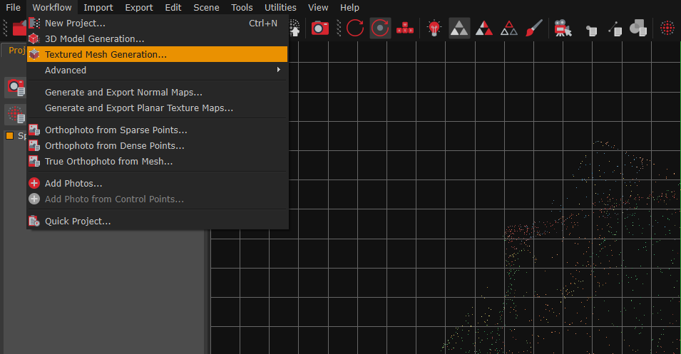
The Textured mesh generation phase can be initiated independently from the New project creation process within the Zephyr workspace by navigating through the Workflow > Textured mesh generation menus. This phase requires a Mesh to be created and listed in the Project tab.
On the Start Reconstruction page, which summarizes the steps and settings chosen during the New Project wizard, it is possible to click the “Run” button to start the Zephyr reconstruction process.

Step 3 – Moving around the reconstruction outcome
After the elaboration process, the “Reconstruction Successful!” dialog will pop up, summarizing the checklist of the correctly oriented cameras in the 3DF Zephyr workspace. Double-clicking the filename will open the appropriate picture in the default image viewer. This is especially useful when dealing with large datasets to quickly identify which cameras weren’t reconstructed successfully. All the cameras and 3D products created during the New Project creation process will be listed on the right in the workspace.
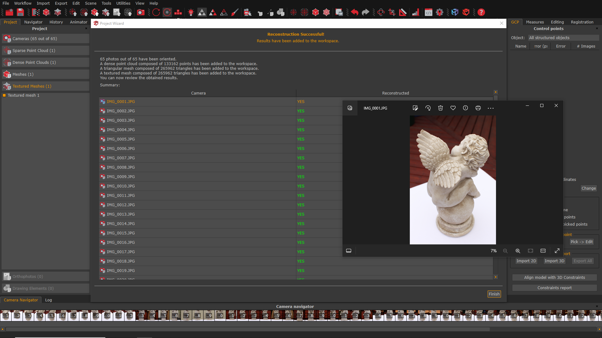
Click the “Finish” button in the right-bottom of the screen. Congratulations!
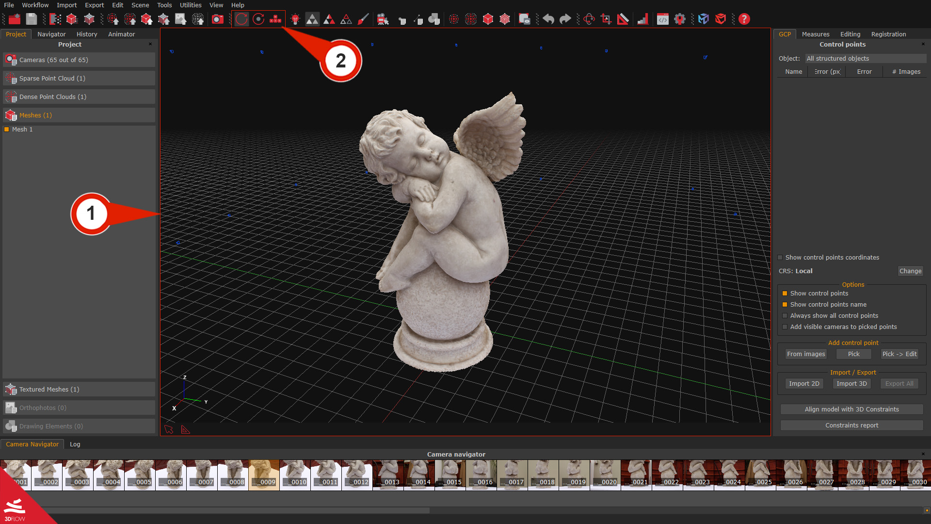
The 3D model is rendered in the center Workspace (1) by default, it is possible to move around the 3D scene using three camera navigation styles. These styles can be enabled from their Icons (2) or by left-clicking on the scene and selecting them in the Camera sub-menu.
| CAMERA STYLE | DESCRIPTION | |
 | Orbit camera | this mode allows hovering the mouse cursor over the scene while holding the left-click and moving the mouse to look around. The mouse wheel can zoom in and out, and pressing Ctrl + left-click while moving the cursor allows panning the view. |
 | Pivot camera | this mode is similar to the previous Orbit mode. However, the pivot is not the center of the reconstruction but is picked on the scene depending on the cursor position each time. |
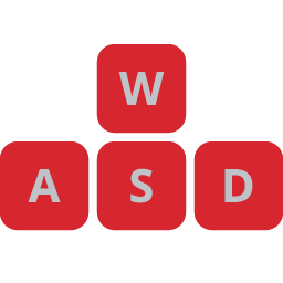 | Free look camera | this mode uses the classic first-person shooter WASD keys. Holding the left mouse button and moving the cursor allows rotating the camera, while the “Q” and “E” keys move up and down, respectively. |
Moving quickly to a camera position in the scene is possible by right-clicking on an image in the Camera list and selecting the “Move here” option. The same action can be performed using the Camera navigator at the bottom of the screen.
Step 4 – Exporting the final mesh
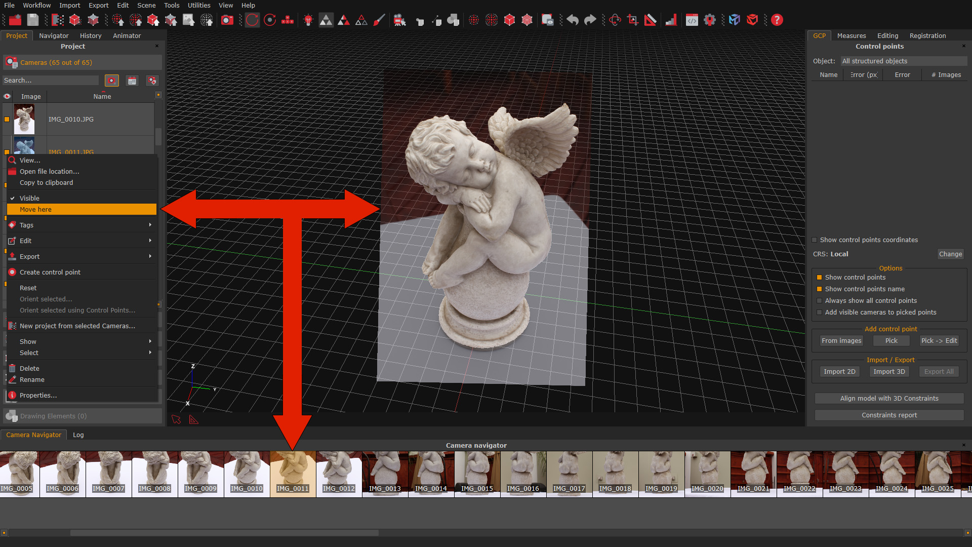
To export the generated Textured mesh, click on the “Export Menu” (1) and then on “Export Textured Mesh” (2). This action will prompt the appearance of the “Textured Mesh Export” (3) window.
Zephyr allows exporting in several file formats. Selecting a specific “Export Format” (4) will unlock the related options in the dialog. In this tutorial, the OBJ/MTL file format is chosen. When ready to export, simply click on the “Export” (5) button in the window’s lower right corner.
Final notes
Opening the exported Cherub mesh in a model viewer of choice should now display an output similar to this below: