
3DF Jimbo – Tutorial
Welcome to the 3DF Zephyr tutorial series. In this tutorial, you will learn how to configure and use 3DF Jimbo. Please note that 3DF Jimbo is available only to selected customers. If you are interested in accessing a 3DF Jimbo license, please contact us at support@3dflow.net using your company/institutional email address.
Getting started with 3DF Jimbo
In this tutorial, you will learn the basic steps to train our segmentation model on your own dataset, so that you can use it for model classification in 3DF Zephyr or, alternatively, for image masking in 3DF Masquerade.
Training a model from pictures in Jimbo requires a dataset of image pairs. Each pair consists of a plain input image and its associated binary mask, in which the desired target is highlighted in white and the background is black. You can use your own dataset by following this tutorial. Note that the image acquisition phase is crucial for successful model training.
A sample dataset is provided so that you can follow along with this tutorial. Please download the “SpaceNet2_Paris.zip” file and extract it on your computer. This dataset consists of 1,148 image pairs (CC-BY-SA 4.0).
 | Download Dataset – Paris2(947MB) |
Step 1 – Load the dataset into Jimbo
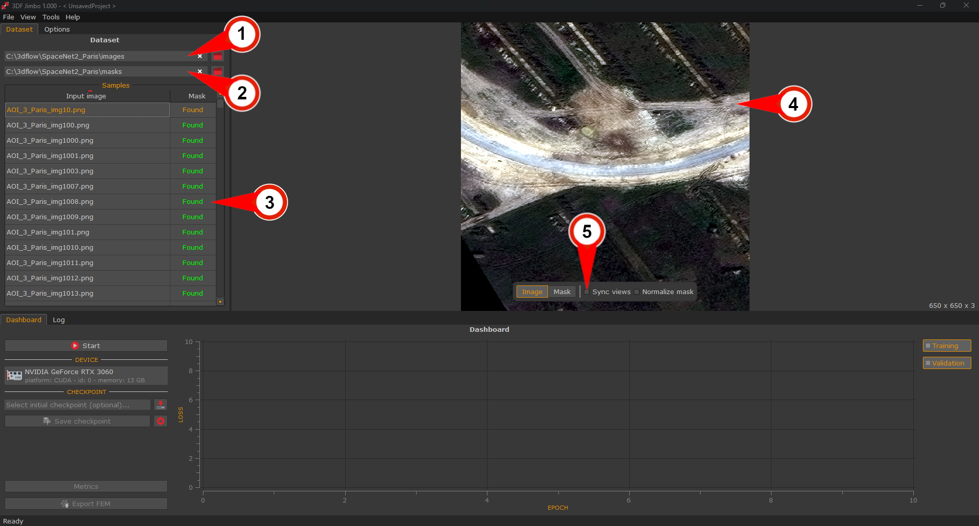
In the “Dataset” section, open the directory containing the input images (1), then open the directory containing the corresponding mask images (2). Jimbo will then automatically pair images and masks based on their file names. Note: images and masks can also be stored in the same folder; in this case, mask file names must follow the same naming convention adopted by 3DF Masquerade in order to be paired correctly. For this tutorial, select the “images” directory as the image directory and the “masks” directory as the mask directory.
In the image list (3), you can check for any unpaired images. By selecting an entry in the list, you can inspect the corresponding pair in the viewer (4). To make inspection easier, you can enable “Sync views” (5) to keep pan and zoom synchronized between the image and its mask.
Step 2 – Configure the training settings
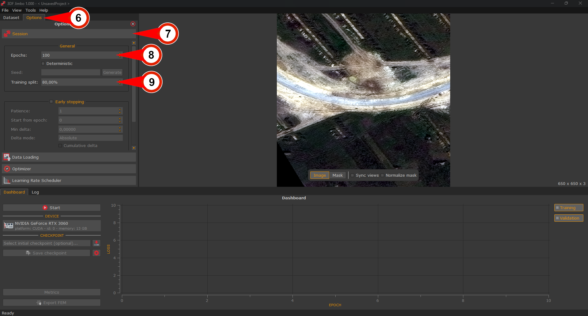
In the “Options” tab (6), you can customize the training session. In particular, in the “Session” subsection (7), you can modify important parameters such as the number of “epochs” (8) and the proportion of the dataset used for the training and testing phases, via the “training split” (9). For this tutorial, set the number of training epochs to 100 and the training split to 80%.
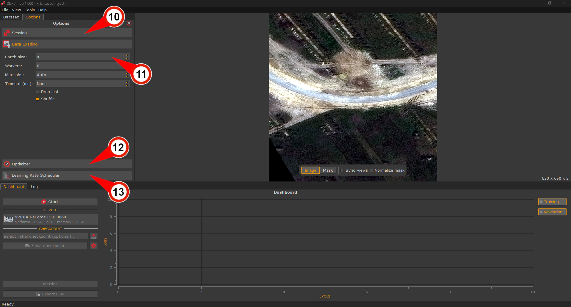
In the “Data loading” subsection (10), you can configure how the dataset is loaded during training. The most important parameter here is the “batch size” (11), which defines how many image pairs are processed together at each training iteration. Larger batches can speed up training, but they require more GPU memory; if your machine runs out of memory during training, lower this value. For this tutorial, set the batch size to 4. You can then adjust it based on your machine’s specifications.
The “Optimizer” subsection (12) lets you choose the algorithm used to update the model’s weights during training, along with its parameters, such as the learning rate. The learning rate controls how large each update step is: a value that is too high can make training unstable, while a value that is too low can make it very slow.
The “Learning Rate Scheduler” subsection (13) defines how the learning rate changes over the course of training. A common strategy is to gradually reduce the learning rate as training progresses, allowing the model to refine its results in the final epochs.
For this tutorial, you can leave the optimizer and scheduler settings at their default values.
Step 3 – Run and monitor the training
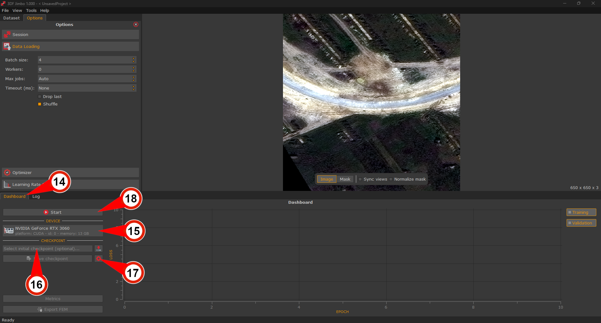
In the “Dashboard” tab (14), you can select the device (15) on which the training will run. Jimbo automatically detects the devices available on your machine and lists them here. If a GPU is available, selecting it will make training considerably faster than running it on the CPU.
Optionally, you can load an initial checkpoint through the file selector (16). A checkpoint stores the model state of a previous training session, so loading one lets you resume training from where it left off instead of starting from scratch. This is not necessary for this tutorial. With the cog button (17), you can set up automatic checkpoint saving, so that the training state is periodically saved during the session. Once everything is set, click the “Start” button (18) to begin training.
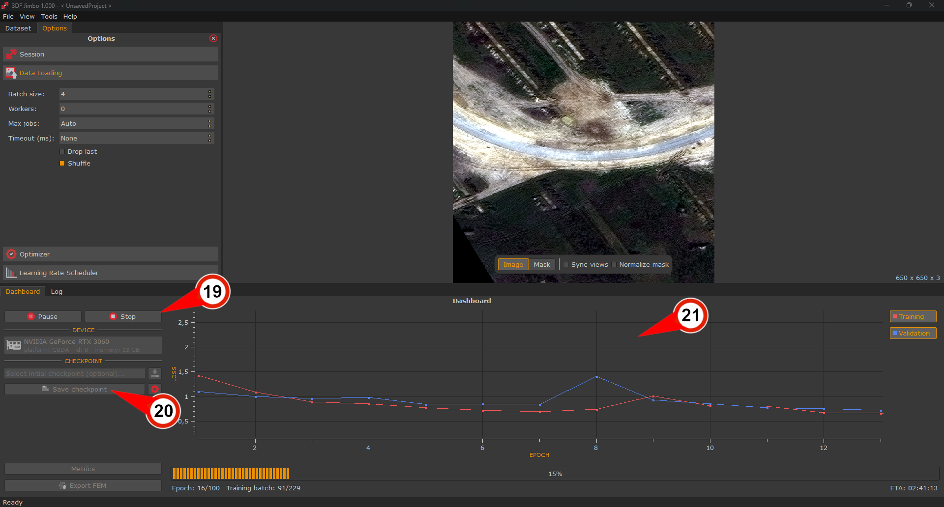
You can pause or stop the training at any time (19). While training is paused, you can manually save a checkpoint to store the model state as it was at the start of the current epoch (20). While training is in progress, you can monitor how the losses evolve in the plot (21).
Step 4 – Export the trained model
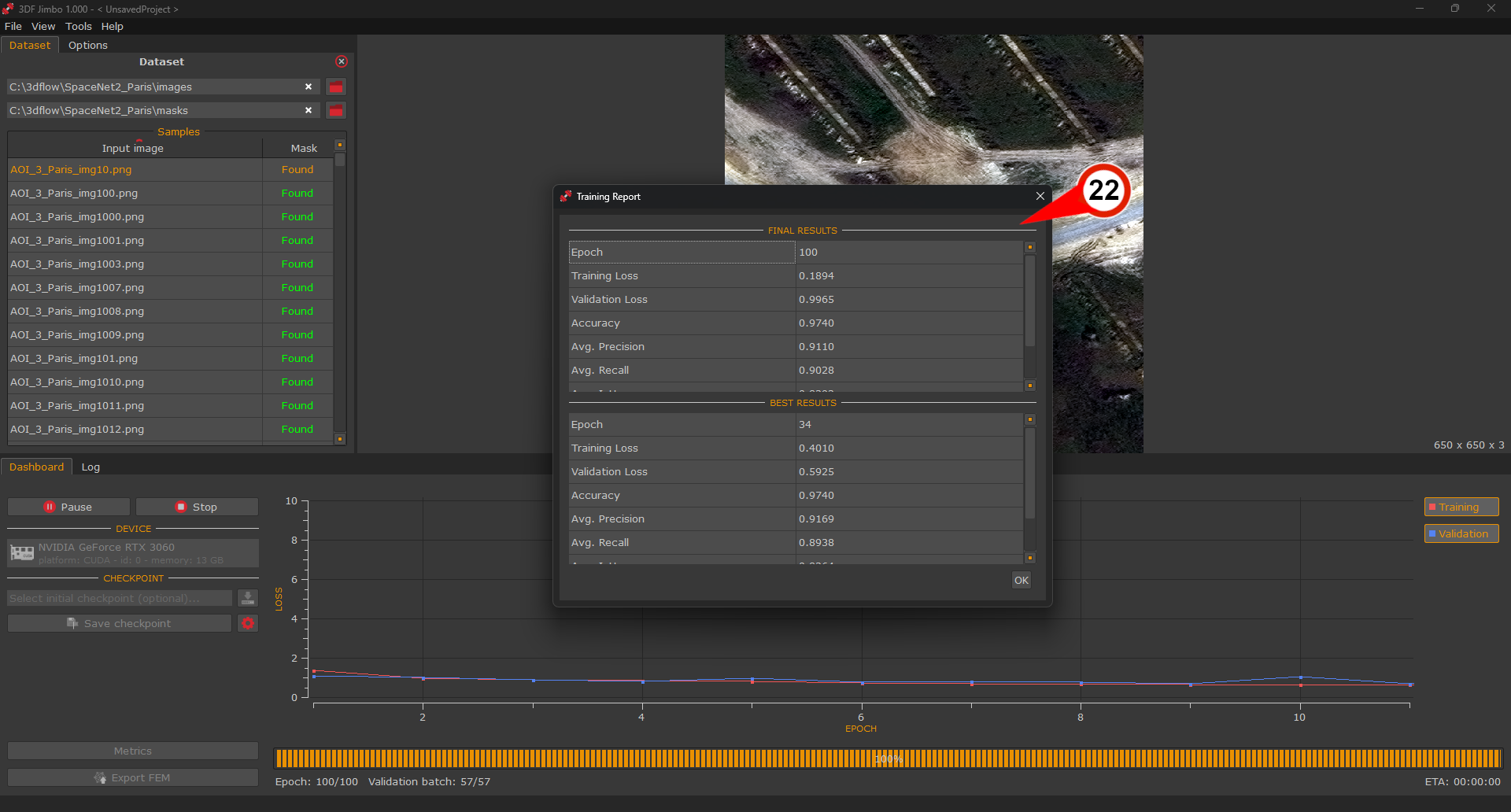
At the end of the training, a dialog (22) will report the statistics of both the final model and the best model. The final model is the one obtained at the last epoch, while the best model is the one that achieved the best results during the training session, which may have been reached before the last epoch.
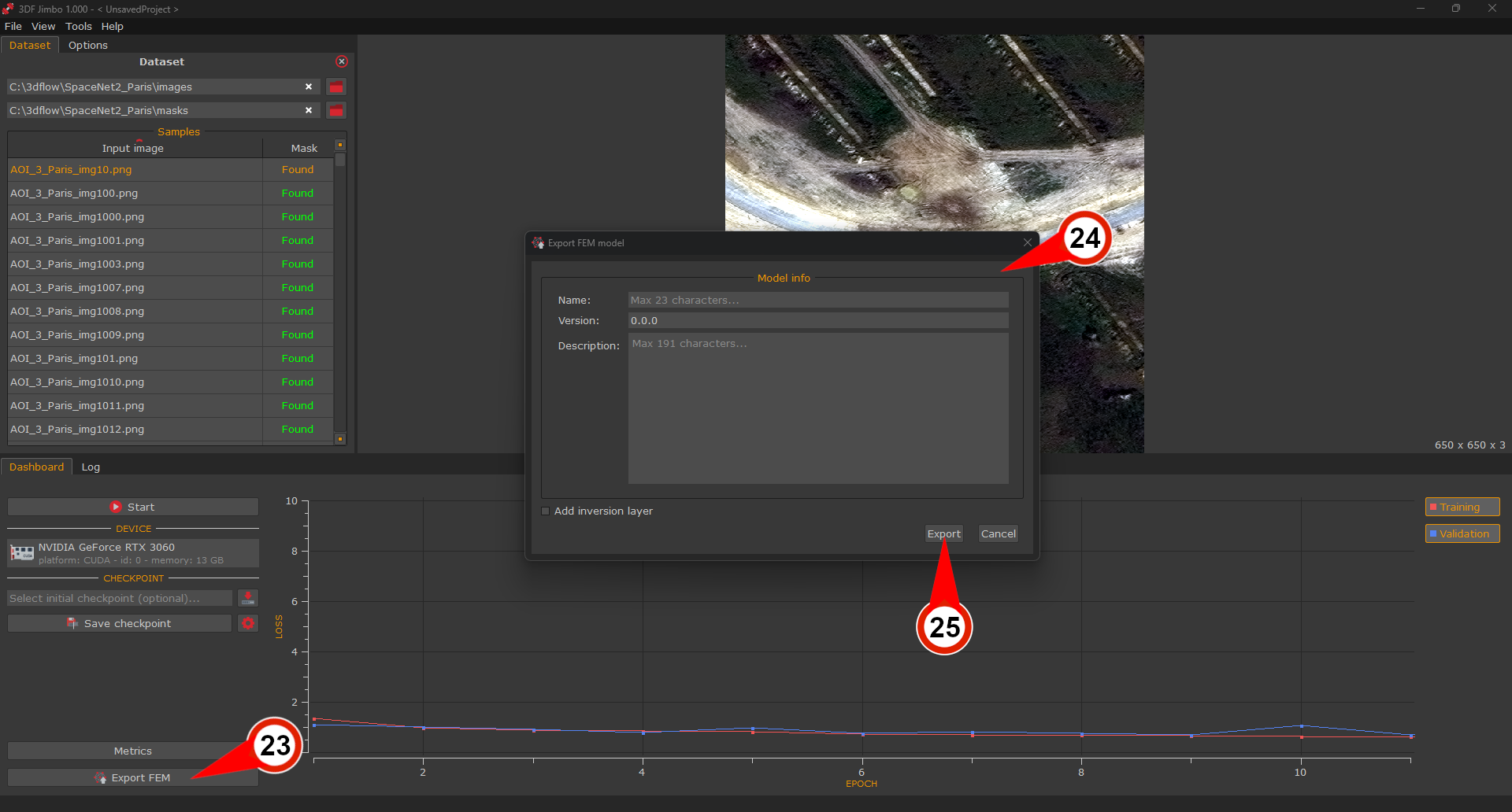
To export the trained model, click the “Export FEM” button (23) in the “Dashboard” tab. In the export dialog (24), you can provide some (optional) information about your model like name, version and brief description. Click “Export” (25) to generate the final model, ready to be used in 3DF Zephyr or 3DF Masquerade.